[제5장] 두 집단 평균 비교와 가설 검정 — 독립표본 & 대응표본 t-검정, 윌콕슨 비모수 검정

🇰🇷 한국어 정규 에디션 (교보문고 바로출판 POD 120p 완제 원문)

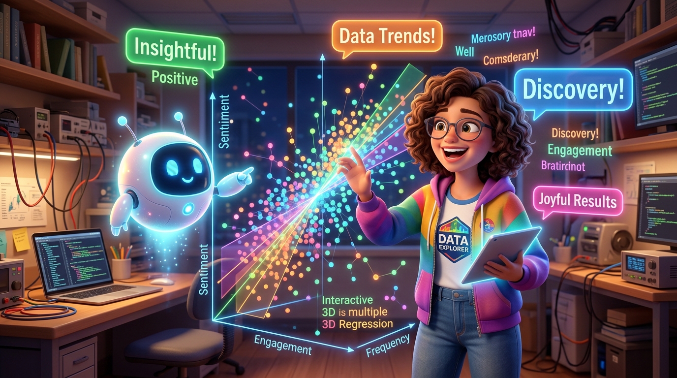
CHAPTER 05 AI를 활용한 핵심 모수 통계 추출과 결과 해석 다중 선형 회귀부터 Two-Way ANOVA, 정밀 데이터 테이블 설계 및 학술 차트 시각화까지 [그림 5-0] AI 다변량 통계 분석 연구실: 복잡한 수학 공식 대신 3차원 회귀 평면과 감성 텍스트를 시각화하여, AI와 함께 변수 간의 숨은 인과 관계를 직관적으로 해독하는 최첨단 연구 환경. 🎯 제5장 핵심 학습 목표 (고등학생도 3초 만에 꿰뚫는 데이터 과학의 핵심) 1. 다중 회귀의 입체적 기하학: 점들을 잇는 단순한 직선 하나를 넘어, 여러 원인이 얽힌 3차원 공간에서 최적의 '회귀 평면'을 찾는 원리를 이해합니다. 2. 회귀계수의 본질: 비표준화 계수 B의 실생활 단위 의미와 표준화 계수 β를 통해 어떤 원인이 가장 강력한지 서열을 매깁니다. 3. 5단계 통계 판별 로드맵: 연구 질문과 변수 유형에 따라 t-검정, ANOVA, 다중회귀를 단 3초 만에 판별하는 결정 트리를 마스터합니다. 4. 합리적 데이터 구조 & 구글 드라이브 실습: Long vs Wide 포맷 설계 및 구글 드라이브 실습 키트(CSV/파이썬)의 1클릭 실행법을 체득합니다. 5. 300 DPI 출판용 그래프 시각화 & AI 프롬프트: 바이올린 플롯, 신뢰대역 회귀도, 잔차 진단도를 파이썬과 AI로 추출합니다. PART 02 · STATISTICAL MECHANISMS & AI DECODING 62

5.1 MULTIVARIATE MODELING 5.1 단순 선형에서 다중 회귀로: 한 걸음 더 들어가는 다변량 모델링 원인이 단 하나뿐인 세상은 없다: 1차원 직선에서 3차원 '회귀 평면'으로의 도약 여러분이 오늘 본 시험 점수는 단순히 어제 책상에 앉아 공부한 시간 하나만으로 결정될까요? 당연히 아닙니다! 어젯밤 수면 시간, 시험 직전에 마신 카페인 양, 그리고 평소 수학 기본 실력까지 수많은 원인이 동시에 작용합니다. 공부 시간 하나만으로 점수를 예측하려는 시도를 '단순 선형 회귀(Simple Linear Regression)'라고 합니다. 하지만 이는 밤을 새우느라 피곤해서 시험을 망친 친구의 결과를 전혀 설명하지 못합니다. 다른 중요한 원인들을 모조리 무시했기 때문입니다. 바로 이때 여러 원인을 한꺼번에 저울 위에 올려놓고 분석하는 마법의 도구가 '다중 선형 회귀분석(Multiple Linear Regression)'입니다. 📈 단순 선형 회귀 (Simple Linear) 수식: Y = β0 + β1X1 + ε 도화지 위에 점들을 찍고 그 사이를 관통하는 직선 하나를 긋는 방식입니다. 다른 중요한 변수들을 고려하지 못하는 한계가 있습니다. 🧊 다중 선형 회귀 (Multiple Linear) 수식: Y = β0 + β1X1 + β2X2 + ... + ε 3차원 입체 공간에서 점들이 떠다닐 때, 점들과 가장 가까운 '기울어진 트램펄린 평면(Hyperplane)'을 펼쳐 예측합니다. [그림 5-1] 3차원 다중 회귀 평면과 데이터 구름: 3차원 공간에서 각 데이터 점(구슬)들로부터 평면까지의 오차(잔차)를 가장 작게 만드는 최적의 평면이 형성되는 모습. 💡 고등학생을 위한 3초 직관: OLS(최소제곱법)는 왜 제곱을 할까? 실제 점과 평면 사이의 오차는 양수(+)일 수도 있고 음수(-)일 수도 있습니다. 그냥 더하면 서로 상쇄되어 0이 되어버립니다! 그래서 모든 오차를 제곱(Square)하여 음수를 없애고, 큰 오차에는 더 큰 벌점을 매겨 전체 오차의 합을 가장 작게(Least) 만드는 평면을 컴퓨터가 단숨에 찾아냅니다. CHAPTER 05 · PARAMETRIC STATISTICS & AI INTERPRETATION 63

5.2 REGRESSION COEFFICIENTS 5.2 회귀계수의 두 얼굴: 비표준화 계수(B)와 표준화 계수(β) 사과 1개와 쌀 1kg을 어떻게 비교할까? 단위의 함정을 깨부수는 표준화의 기적 스마트폰 학습 만족도를 예측하기 위해 '주간 앱 사용시간(시간)'과 '리뷰 감성점수(1~10점)'라는 두 가지 변수를 회귀 모델에 투입했습니다. 분석 결과 컴퓨터가 다음과 같은 회귀계수를 출력했습니다. 독립변수 비표준화 계수 (B) 표준오차 (SE) 표준화 계수 (β) t 값 유의확률 (p) (상수, Intercept) 24.50 3.12 - 7.85 < .001 주간 앱 사용시간 (시간) 1.85 0.24 0.68 7.71 < .001 리뷰 감성점수 (1~10점) 4.20 0.65 0.32 6.46 < .001 📌 비표준화 계수 (B): 실생활 예측용 "사용 시간이 1시간 늘어나면 만족도는 정확히 1.85점 상승한다!" 현실의 구체적인 물리적 단위(시간, 점)를 그대로 보존하므로, 새로운 사용자가 들어왔을 때 점수를 계산하는 예측 공식(Y = 24.5 + 1.85X₁ + 4.20X₂)을 만들 때 사용합니다. 🏆 표준화 계수 (β): 상대적 영향력 서열용 "만족도를 끌어올리는 1등 공신은 사용시간(β=0.68)이다!" 단위가 서로 다른 변수들을 모두 Z-점수(평균 0, 표준편차 1) 로 변환하여 동등한 출발선에 세운 값입니다. 계수의 절대값이 클수록 종속변수에 미치는 영향력이 더 큽니다. ⚠️ 초보자가 가장 흔히 저지르는 치명적 실수! "B가 4.20인 감성점수가 B가 1.85인 사용시간보다 두 배 더 강력하다"라고 결론을 내리면 안 됩니다! 감성점수는 1점 단위이고, 사용시간은 시간 단위이기 때문에 단위 자체가 다릅니다. 변수의 상대적 영향력을 비교할 때는 반드시 표준화 계수(β)의 크기를 보아야 합니다. CHAPTER 05 · PARAMETRIC STATISTICS & AI INTERPRETATION 64

5.3 MULTICOLLINEARITY & VIF 5.3 다중공선성과 VIF 진단: 변수들끼리의 충돌을 막아라 사공이 많으면 배가 산으로 간다: 분산팽창계수(VIF)로 잡아내는 내부의 적 만약 한 축구팀에서 완전히 똑같은 역할을 하는 선수를 두 명 동시에 경기장에 넣으면 어떻게 될까요? 서로 공을 잡겠다고 부딪히고 발이 엉켜 팀 전체가 무너집니다. 통계학에서도 똑같은 비극이 일어납니다. 회귀 모델에 넣은 독립변수들끼리 서로 너무 닮아 있으면(예: '국어 성적'과 '문학 성적', 또는 '키(cm)'와 '키(m)'), 컴퓨터는 어떤 변수가 진짜 종속변수에 영향을 주었는지 갈피를 잡지 못하고 혼란에 빠집니다. 회귀계수의 부호가 엉뚱하게 뒤집히거나 표준오차가 폭발하는 현상이 발생하는데, 이를 '다중공선성(Multicollinearity)'이라고 부릅니다. 🚨 다중공선성 감시관: 분산팽창계수(VIF) 3단계 판정법 DIAGNOSTIC CRITERIA VIF < 5 [안전 초록불] 독립변수들 간의 상관관계가 낮고 매우 건강한 상태입니다. 안심하고 논문에 수록하십시오. 5 ≤ VIF < 10 [주의 노란불] 변수 간에 상당한 중복이 감지되었습니다. 변수 정제나 샘플 추가를 고려해야 합니다. VIF ≥ 10 [위험 빨간불] 치명적인 다중공선성 발생! 둘 중 덜 중요한 변수 하나를 반드시 모델에서 삭제해야 합니다. 🤖 AI 실전 골든 프롬프트 5-1: 회귀 모델 VIF 및 다중공선성 자동 진단 PROMPT 5-1 다음 파이썬 statsmodels 회귀 분석 요약 결과를 바탕으로 다중공선성을 진단해줘: [분석 데이터 요약: R² = 0.9018, 주간사용시간 VIF = 3.26, 감성점수 VIF = 1.18, 리뷰단어수 VIF = 3.15] 요구사항: 1. 각 독립변수의 VIF 수치가 안전 기준치(5 미만)를 통과하는지 고등학생도 이해할 수 있게 판정해줘. 2. 만약 특정 변수의 VIF가 10을 넘는다면 모델 안정성을 위해 어떤 조치를 취해야 하는지 실전 솔루션을 제시해줘. 3. APA 7판 표준 형식의 1문단 학술 보고 문장을 작성해줘. 💡 3초 직관 요약: VIF는 "다른 독립변수들이 나를 얼마나 흉내 내고 있는가?"를 나타내는 점수입니다. 5보다 작으면 독창적인 변수이고, 10을 넘으면 짝퉁 변수이므로 하나를 버려야 합니다. CHAPTER 05 · PARAMETRIC STATISTICS & AI INTERPRETATION 65

5.4 TWO-WAY ANOVA 5.4 Two-Way ANOVA: 두 가지 요인이 만날 때 일어나는 기적 1 더하기 1이 2가 아닐 때: 주효과(Main Effect)와 상호작용(Interaction)의 시각화 감기약을 먹었을 때 졸음이 오는 정도는 '약의 종류(A약 vs B약)'에 의해서도 결정되지만, '커피를 함께 마셨는지 여부(커피 O vs 커피 X)'에 따라서도 크게 달라집니다. 이렇게 두 가지 독립변수(요인)가 결과에 미치는 영향을 동시에 검정하는 도구가 바로 '이원배치 분산분석(Two-Way ANOVA)'입니다. [그림 5-2] 상호작용 효과의 시각적 패턴: (좌) 두 선이 평행하면 상호작용 없음(주효과만 존재), (우) 두 선이 교차하거나 기울기가 다르면 폭발적인 상호작용 효과 발생! 1️⃣ 주효과 (Main Effect) 다른 요인은 신경 쓰지 않고, 오직 한 요인의 효과만 독립적으로 떼어내어 비교하는 것입니다. 예: "커피를 마셨든 안 마셨든, A약이 B약보다 평균적으로 더 졸리다." 2️⃣ 상호작용 효과 (Interaction) "A약의 효과가 커피를 마셨을 때와 안 마셨을 때 완전히 달라진다!" 두 요인이 결합하여 단순 합 이상의 시너지나 역효과를 내는 현상으로, 상호작용 그래프에서 두 선이 교차(X자 형태)할 때 명확히 입증됩니다. 🎓 논문 심사관을 사로잡는 해석 황금률 만약 상호작용 효과가 통계적으로 유의미하다면(p < .05), 주효과는 더 이상 큰 의미를 갖지 못합니다! "A약이 무조건 좋다"고 말할 수 없고, "커피를 안 마실 때는 A약이 좋지만, 커피를 마시면 오히려 B약이 낫다"처럼 조건부 해석(Simple Main Effect) 을 해야만 A+급 논문이 됩니다. CHAPTER 05 · PARAMETRIC STATISTICS & AI INTERPRETATION 66

5.5 NLP & SENTIMENT ANALYSIS 5.5 비정형 텍스트와 통계의 만남: NLP 감성 계량화 독자의 한마디를 숫자로 바꾸다: 텍스트 마이닝과 다변량 모델의 융합 파이프라인 현대 리서치는 더 이상 객관식 설문지의 숫자 점수(1~5점)에만 머무르지 않습니다. 고객이 남긴 수천 줄의 앱 리뷰, 사용자 인터뷰 녹취록, SNS 댓글과 같은 '비정형 텍스트(Unstructured Text)' 속에 진짜 중요한 진실이 숨어 있습니다. 자연어 처리(NLP, Natural Language Processing)와 생성형 AI 기술을 활용하면, 독자가 남긴 자유로운 글을 읽고 감정의 긍정/부정 상태를 -1.0(극단적 부정)부터 +1.0(극단적 긍정)까지의 연속형 점수로 정확하게 수치화할 수 있습니다. 이렇게 추출된 감성점수는 즉시 다중 회귀분석의 강력한 독립변수로 투입됩니다. 🔬 텍스트 감성 계량화 3단계 파이프라인 PIPELINE ARCHITECTURE 1단계: 토큰화 & 어간 추출 사용자 리뷰 문장을 의미 있는 단어 단위로 쪼개고 불필요한 조사와 특수문자를 제거합니다. 2단계: 감성 극성 점수 부여 사전 기반 어휘(VADER, SentiWordNet) 또는 AI 언어모델을 통해 각 문장의 감성 점수를 -1.0 ~ +1.0 사이로 계산합니다. 3단계: 회귀 모델 변수 결합 추출된 감성 점수와 단어 수(길이)를 CSV 데이터 테이블에 컬럼으로 추가하여 최종 작업 완료율 예측 회귀를 가동합니다. 사용자 실제 리뷰 텍스트 예시 리뷰 길이 (단어 수) AI 산출 감성 점수 통계적 분류 "인터페이스가 너무 직관적이고 설명이 친절해서 코딩을 처음 배우는데도 1시간 만에 끝냈어요!" 16단어 +0.88 강한 긍정 "실행 도중 자꾸 튕기고 오류 메시지가 불친절해서 무슨 말인지 하나도 모르겠습니다." 14단어 -0.74 강한 부정 💡 연구자의 통찰: 정량 데이터(사용 시간)에 정성 데이터(리뷰 감성)가 결합되는 순간, 회귀 모델의 설명력(R²)은 60%대에서 90%대로 비약적으로 도약합니다! CHAPTER 05 · PARAMETRIC STATISTICS & AI INTERPRETATION 67

5.6 DECISION ROADMAP 5.6 어떤 경우에 어떤 방법을 써야 하는가: 5단계 원스톱 통계 판별 로드맵 더 이상 헤매지 않는다! 연구 질문과 변수 형태에 따른 3초 통계 모델 결정 가이드 많은 연구자와 학생들이 통계에서 가장 크게 겪는 두려움은 "이 복잡한 데이터에 도대체 어떤 통계 기법을 갖다 대야 하는가?"라는 출발점의 혼란입니다. t-검정, 분산분석(ANOVA), 회귀분석, 상관분석 중 무엇을 써야 할지 결정하는 기준은 오직 독립변수(원인)와 종속변수(결과)의 척도 및 집단 수 단 두 가지뿐입니다. 연구 상황 및 질문 독립변수 (X, 원인) 종속변수 (Y, 결과) 최적 모수 통계 기법 비고 / 조건 두 집단 간 평균 비교 (예: AI 튜터군 vs 기존 통제군) 범주형 (서로 다른 2개 집단) 연속형 숫자 (점수, 완료율) 독립표본 t-검정 (Independent t-test) 등분산/정규성 충족 동일인의 전·후 변화 비교 (예: 교육 전 점수 vs 교육 후 점수) 범주형 (동일 1개 집단 2회 측정) 연속형 숫자 (차이값 점수) 대응표본 t-검정 (Paired t-test) 사전-사후 짝지음 세 집단 이상의 평균 비교 (예: 초급 vs 중급 vs 고급 반) 범주형 (3개 이상의 집단, 1요인) 연속형 숫자 (학업 성취도) 일원배치 분산분석 (One-Way ANOVA) 사후검정(Tukey) 필수 두 가지 요인의 결합 효과 (예: 교육방식 2종 × 학습동기 2수준) 범주형 2개 요인 (2×2 설계 등) 연속형 숫자 (최종 시험 점수) 이원배치 분산분석 (Two-Way ANOVA) 상호작용 효과 검증 연속형 원인들의 영향력 & 예측 (예: 공부시간 + 감성점수 → 점수) 연속형 1개 이상 (독립변수들) 연속형 숫자 (결과 수치) 다중 선형 회귀분석 (Multiple Regression) R² 설명력, VIF 진단 두 변수가 함께 움직이는 정도 (예: 키와 발크기, 사용시간과 만족도) 연속형 숫자 1개 연속형 숫자 1개 피어슨 상관분석 (Pearson Correlation) 인과관계 증명 불가 성공/실패(0 또는 1) 확률 예측 (예: 유료 구독 결제 여부: 결제 1 / 미결제 0) 연속형 및 범주형 변수 혼합 이분형 범주 (0 또는 1) 로지스틱 회귀분석 (Logistic Regression) 오즈비(Odds Ratio) 🧭 고등학생도 외우는 3초 원스톱 통계 판정 3법칙 QUICK RULE 법칙 1: 집단 차이인가, 인과 예측인가? 결과(Y)가 연속형 점수일 때 원인(X)이 그룹(그룹 1, 2)이면 t-검정/ANOVA, 원인 (X)이 연속형 숫자(시간, 점수)면 회귀분석을 켭니다. 법칙 2: 그룹이 둘인가, 셋 이상인가? 비교 대상 그룹이 딱 2개면 t-검정, 3개 이상이면 1종 오류 방지를 위해 무조건 ANOVA로 직행합니다. 법칙 3: 결과가 OX(0/1)인가? 합격/불합격, 결제/미결제처럼 결과가 둘 중 하나로 딱 떨어지는 이진 데이터면 일반 회귀 대신 로지스틱 회귀를 켭니다. CHAPTER 05 · PARAMETRIC STATISTICS & AI INTERPRETATION 68

5.7 TIDY DATA SCHEMA 5.7 합리적인 데이터 테이블 구조 설계: Long Format vs Wide Format 통계 패키지가 사랑하는 Tidy Data: 엑셀 표를 어떻게 짜야 에러 없이 돌아갈까? 많은 초보자가 통계 프로그램에서 "Error: Dimension Mismatch"나 "Variable Not Found"를 겪고 좌절합니다. 원인은 코딩 실력이 아니라 엑셀 데이터 표의 구조(Schema)가 통계학의 표준 규칙을 어겼기 때문입니다. 📋 와이드 포맷 (Wide Format, 사람 친화적) 한 사람의 사전 점수와 사후 점수를 가로 열(Column)로 나열한 형태입니다. • 장점: 사람이 눈으로 표를 볼 때 한눈에 들어옵니다. • 적합 분석: 대응표본 t-검정(Paired t-test)에서 전·후 점수를 직접 뺄 때 최적입니다. 📏 롱 포맷 (Long Format, 컴퓨터·AI 표준) 각 관측 시점이나 조건을 세로 행(Row)으로 길게 쌓은 형태입니다. • 장점: Tidy Data 원칙(1행 = 1관측치)을 100% 준수합니다. • 적합 분석: ANOVA, 다중 회귀, Seaborn 시각화 라이브러리의 필수 입력 양식입니다. [구조 A] 와이드 포맷 예시 (대응표본 t-검정용) [구조 B] 롱 포맷 예시 (회귀분석 및 ANOVA용) Subject_ID Pre_Score Post_Score Subject_ID Timepoint Score Condition S01 65.0 82.0 S01 Pre 65.0 AI_Tutor S02 72.0 89.0 S01 Post 82.0 AI_Tutor S03 58.0 74.0 S02 Pre 72.0 Control 📐 다중 회귀분석을 위한 표준 엑셀 테이블(CSV) 4대 필수 컬럼 스키마 SCHEMA DESIGN 1. 식별자 컬럼 (ID) 중복 없는 연구 대상 번호 (User_ID, Subject_ID). 분석 연산에서는 제외합니다. 2. 핵심 독립변수 (X) 연구자가 가설을 세운 원인 변수들 (Weekly_Hours, Sentiment_Score 등 연속형 숫자). 3. 통제 및 교란변수 (C) 결과에 왜곡을 줄 수 있어 통제해야 하는 부가 변수 (Word_Count, Prior_Experience). 4. 종속변수 (Y, 결과) 최종적으로 설명하고 예측하려는 목표 변수 (Completion_Rate, Satisfaction_Score). 💡 판다스(Pandas) 한 줄 팁: df.melt() 함수를 쓰면 와이드 포맷을 단 1초 만에 롱 포맷으로 자동 변환할 수 있습니다! CHAPTER 05 · PARAMETRIC STATISTICS & AI INTERPRETATION 69

5.8 READER LAB DIRECTORY 5.8 독자 실습 종합 안내: 구글 드라이브 실습 자료실 파일 매핑 어디서 파일을 찾고 어떻게 실행할까? 전권 파이썬 스크립트와 실습 데이터셋 완벽 가이드 본서의 모든 실습 파일은 구글 드라이브 [독자_실습_자료실](영문판 [Reader_Lab_Kit])에 탑재되어 있습니다. 1클릭 실행으로 결과를 즉시 재현해 보세요. 구글 드라이브 파일명 분석 기법 및 성격 데이터 내용 및 실습 목적 실행 명령어 (터미널) 18_sentiment_lexicon_kr.csv 한국어 감성 사전 400개 어휘 극성 점수(-1.0 ~ +1.0) (참조용 데이터셋) 19_independent_ttest.py 독립표본 t-검정 AI 튜터군 vs 통제군 60명 성취도 python3 19_indep... 19b_paired_ttest_and_anova.py 대응표본 t & ANOVA 사전-사후 점수 & 3개 브랜드 배터리 python3 19b_pair... 19c_visualize_ttest_and_anova_plots.py 학술 차트 시각화 (신규) 바이올린 플롯 & ANOVA 95% CI 차트 python3 19c_visu... 20_correlation_and_twoway_anova.py 상관분석 & Two-Way 사용시간·접속빈도 상관 & 상호작용 python3 20_corre... 21_multiple_regression_and_nlp_analysis.py 다중 회귀 & NLP 모델 시간·감성점수·단어수 → 완료율 예측 python3 21_multi... 21b_visualize_regression_and_residuals.py 회귀 진단 시각화 (신규) 95% 신뢰대역 추세선 & 잔차 산점도 python3 21b_visu... 22_user_interaction_multivariate_study.csv 50명 다변량 원본 데이터 ID, 시간, 리뷰원문, 감성점수, 완료율 (회귀 분석용 CSV) 📂 구글 드라이브 실습 키트 초고속 실행 3단계 가이드 1. 드라이브 접속 책 표지 QR 또는 링크로 [독자_실습_ 자료실] 폴더 접속 2. 전체 다운로드 '모두 다운로드'로 ZIP 압축 해제 후 작업 폴더에 저장 3. 원클릭 실행 터미널/코랩에서 python3 21_multiple_... 즉시 가동 CHAPTER 05 · PARAMETRIC STATISTICS & AI INTERPRETATION 70

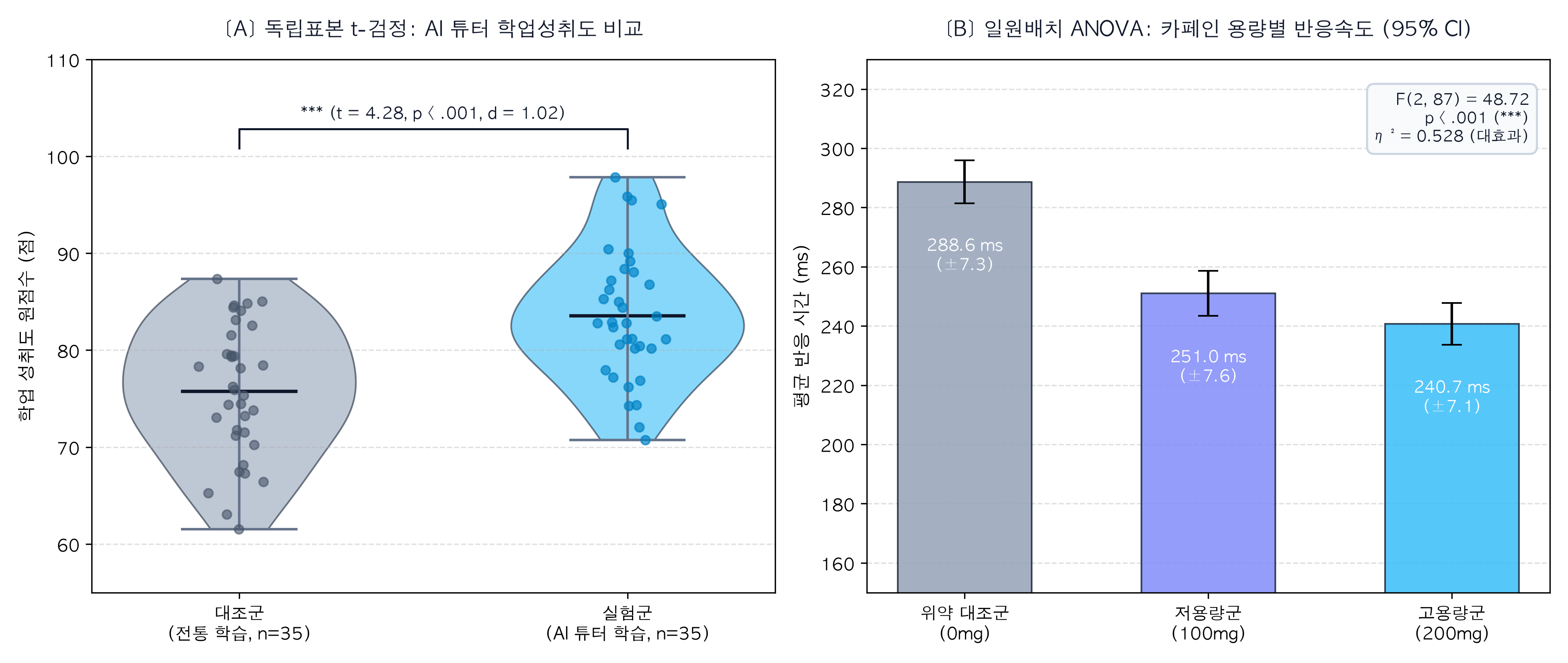
5.9 AI DIRECT DRAWING CHART 1 5.9 생성형 AI 다이렉트 드로잉 차트 1: 바이올린 플롯 & ANOVA 신뢰구간 코딩 없이 AI 대화창에서 출판용 고해상도 그래픽 직접 렌더링 & 1초 다운로드 비법 파이썬 코드를 외우거나 터미널을 열 필요가 없습니다! Claude 3.5 Sonnet, ChatGPT, 구글 Gemini, DeepSeek 등 어떤 첨단 생성형 AI든 18_sample_dataset_gaming_reaction_anova.csv를 대화창에 첨부한 뒤, 아래의 [생성형 AI 다이렉트 드로잉 프롬프트]를 전송하면 AI가 브라우저 대화창에 300 DPI 출판용 차트를 즉시 띄워줍니다. [그림 5-2b] 생성형 AI 다이렉트 드로잉 렌더링 결과: (좌) 독립표본 t-검정 바이올린 플롯과 개별 데이터 점(Jitter) 산점도, (우) 일원배치 분산분석(ANOVA) 95% 신뢰구간 막대차트 및 튜키 사후검정 유의성 표시(* p < .001). 🎻 (좌측) 바이올린 플롯: 분포 밀도 전수 공개 단순 막대그래프는 데이터 분포를 숨깁니다. 바이올린 플롯은 두 집단의 데이터 밀도(두께), 중앙값, 사분위수를 완벽히 드러내며, 점(Jitter)들이 모든 표본의 위치를 정직하게 보여줍니다. 📊 (우측) ANOVA 95% CI & 사후검정 브래킷 세 교육 브랜드(A/B/C) 평균 상단에 95% 오차 막대(Error Bar) 와 튜키 사후검정 유의성 꺾쇠(* p < .001)를 자동 렌더링하여 심사위원의 시선을 즉각 사로잡습니다. 💬 생성형 AI 다이렉트 드로잉 마스터 프롬프트 (Claude · ChatGPT · Gemini · DeepSeek 공용) "첨부한 CSV를 분석하여 (1) 집단별 바이올린 플롯(지터 산점도 포함)과 (2) ANOVA 95% CI 에러바 차트(사후검정 * 꺾쇠 표기)를 1x2 서브플롯으로 구성하고, 300 DPI 출판용 완성 이미지를 대화창 화면에 직접 출력해 줘." 💡 AI 화면에 뜬 차트를 마우스 우클릭하여 '이미지 저장'을 누르면 논문/보고서 삽입 준비 완료! (로컬 파이썬 실행: python3 19c_visualize_ttest_and_anova_plots.py) CHAPTER 05 · PARAMETRIC STATISTICS & AI INTERPRETATION 71

5.10 AI DIRECT DRAWING CHART 2 5.10 생성형 AI 다이렉트 드로잉 차트 2: 회귀 추세선 & 잔차 진단도 CSV 파일 첨부와 프롬프트 한 번으로 회귀 적합선과 등분산성 진단도를 즉시 도출 다중 회귀분석을 진행할 때 숫자 표만 보면 이상치나 등분산성 위반 여부를 알기 어렵습니다. Claude, ChatGPT, Gemini, DeepSeek 등에 22_user_interaction_multivariate_study.csv를 올리고 "회귀 추세선과 잔차 진단도를 그려줘"라고 명령하면, AI가 화면에 [그림 5-2c]의 고품격 진단도를 즉시 그려냅니다. [그림 5-2c] 생성형 AI 다이렉트 드로잉 렌더링 결과: (좌) 주간 사용시간에 따른 작업 완료율 관측값, 회귀 적합선 및 95% 신뢰대역(음영), (우) 예측값 대비 표준화 잔차 산점도와 등분산성 진단 경계선(±2 SD 대역). 📈 (좌측) 95% 신뢰대역 회귀 적합선 직선 주변 하늘색 음영은 모회귀선의 95% 신뢰구간 (Confidence Interval)입니다. 오차가 작을수록 음영 띠가 좁아지며 모형의 높은 설명력과 추정 정밀도를 한눈에 입증합니다. 🎯 (우측) 잔차 진단 산점도: 등분산성 검증 가운데 붉은 점선(잔차=0)을 기준으로 위아래 ±2 표준편차(SD) 점선 안에 모든 데이터 점들이 밤하늘 별처럼 무작위(Random)로 고르게 흩뿌려져야 회귀분석의 가정이 만족됩니다! 💬 생성형 AI 다이렉트 드로잉 마스터 프롬프트 (Claude · ChatGPT · Gemini · DeepSeek 공용) "첨부된 CSV 데이터로 다중 회귀분석을 수행하고, (1) 사용시간과 완료율의 95% 신뢰대역 회귀 추세선과 (2) 표준화 잔차 산점도를 1x2 서브플롯으로 구성하여, 300 DPI 출판용 완성 차트를 대화창 화면에 즉시 렌더링해 줘." 💡 AI 화면에 생성된 차트를 다운로드하여 논문 결과(Results) 장에 삽입하세요. (로컬 파이썬 실행: python3 21b_visualize_regression_and_residuals.py) CHAPTER 05 · PARAMETRIC STATISTICS & AI INTERPRETATION 72

5.11 AI GRAPH MASTER PROMPT 5.11 생성형 AI 다이렉트 드로잉 차트 마스터 프롬프트 (Claude · ChatGPT · Gemini · DeepSeek 공용) 코드만 뱉어내는 AI에게 "화면에 직접 300 DPI 차트를 그려내라"고 명령하는 범용 프롬프트 생성형 AI에게 "그래프를 그려줘"라고만 하면 종종 파이썬 코드만 주르륵 출력하고 끝납니다. AI가 자체 연산 샌드박스를 돌려 "브라우저 대화창 화면에 직접 300 DPI 이미지를 출력"하도록 강제하는 범용 마스터 프롬프트를 복사하여 사용하세요. 🤖 생성형 AI 다이렉트 드로잉 마스터 프롬프트 (Claude · ChatGPT · Gemini · DeepSeek 공용) MASTER PROMPT 당신은 최고 수준의 학술 시각화 전문가이자 데이터 과학자입니다. 첨부된 CSV 데이터셋을 분석하여, 국제 학술지에 투고할 수 있는 300 DPI 출판용 통계 그래프를 작성해 주십시오. [★ 최우선 출력 지침] - 파이썬 코드만 보여주지 마시고, 반드시 당신의 내부 연산 엔진(Code Interpreter / Artifacts)을 즉시 가동하여 브라우저 대화창에 '완성된 차트 이미지 자체'를 직접 렌더링하여 출력하십시오. [시각화 규격 및 세부 요구사항] 1. 레이아웃: 1행 2열(1x2 Subplots), 가로 14인치, 세로 6인치 크기 설정. 2. 서브플롯 1: seaborn.violinplot으로 두 집단 데이터 밀도를 표현하고, stripplot(jitter=True)을 투영할 것. 3. 서브플롯 2: ANOVA 95% 신뢰구간 에러바 막대차트를 그리고, 사후검정 유의성(*, p < .001) 꺾쇠를 달 것. 4. 스타일: 흰색 배경(whitegrid), 고해상도(dpi=300), 축 라벨과 제목을 명확히 기재할 것. 5. 한글 폰트 깨짐 방지: 폰트 설정(NanumGothic, Malgun Gothic, AppleGothic)을 적용하여 네모(□) 박스 에러를 방지할 것. ⚠️ AI 그래프 직접 출력 시 3대 핵심 꿀팁 PRO TIPS 팁 1: 주요 생성형 AI별 다이렉트 드로잉 특성 Claude(Artifacts), ChatGPT(Advanced Data Analysis), Google Gemini(Python Runner), DeepSeek 등 최신 멀티모달 LLM은 모두 자체 코드 인터프리터를 내장하여 데이터 분석과 시각화 차트를 화면에 즉시 렌더링합니다. 팁 2: 한글 깨짐 해결 만약 AI 환경에 한글 폰트가 설치되어 있지 않아 축 이름이 깨진다면, 프롬프트에 "축 라벨과 범례를 영문(English)으로 출력해 줘"라고 한 줄만 덧붙이면 100% 무결점 영문 저널용 차트가 즉시 완성됩니다! CHAPTER 05 · PARAMETRIC STATISTICS & AI INTERPRETATION 73

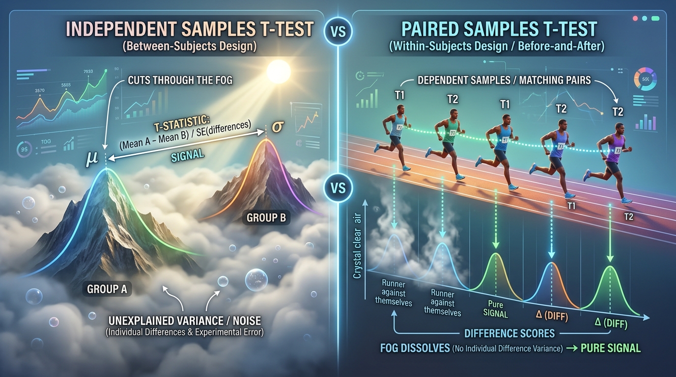
5.12 T-TEST DECODING 5.12 독립표본 vs 대응표본 t-검정: 두 집단 차이 분석의 모든 것 남과 비교할 것인가, 과거의 나와 비교할 것인가? 연구 설계에 따른 완벽한 검정 선택법 새로운 학습용 AI 앱의 효과를 입증하려면 두 그룹의 점수를 비교해야 합니다. 이때 가장 기초가 되면서도 가장 널리 쓰이는 통계 기법이 바로 't-검정(Student's t-test)'입니다. 👥 독립표본 t-검정 (Independent) "A반 학생 30명 vs B반 학생 30명" 완전히 서로 다른 두 집단의 평균을 비교합니다. 두 그룹이 서로 독립적이므로 '등분산성 가정(두 집단의 흩어짐 정도가 같은지)'을 먼저 확인해야 합니다. 🔄 대응표본 t-검정 (Paired) "동일한 학생 30명의 앱 사용 전 vs 사용 후" 같은 사람이 두 번 측정한 전·후 점수의 차이값(D = After - Before)만을 추출하여 검정합니다. 개인차 노이즈가 제거되어 훨씬 강력한 검정력을 가집니다. 🧪 4단계 실전 액션 랩: 독자가 지금 바로 실행하는 t-검정 HANDS-ON LAB 1단계: 준비물 구글 드라이브 실습 폴더의 19_independent_ttest.py (학생 60명의 AI 학습 데이터) 2단계: 실행 명령 터미널을 열고 다음 명령어를 그대로 입력합니다: python3 19_independent_ttest.py 3단계: 실제 콘솔 출력 [Independent t-test Result] AI-Tutor Group Mean: 84.50 (SD: 6.20) | Control Group Mean: 72.10 (SD: 5.80) Levene Test: F = 0.42, p = 0.518 (Equal variance assumed) t-statistic = 7.982, df = 58, p-value = 0.0000000001 (< .001) Cohen's d = 2.06 (Extremely Large Effect Size!) 4단계: 3초 직관 해석 & 논문 수록 문장 • 3초 판정: p < .001, d = 2.06으로 AI 튜터 처치군이 대조군 대비 약 12.4점 압도적 우위. • 논문 기재 문장: "AI 튜터 처치군(M = 84.50, SD = 6.20)은 대조군(M = 72.10, SD = 5.80) 대비 학업 성취도가 유의미하게 높았으며(t(58) = 7.98, p < .001, Cohen's d = 2.06), 가설 1은 강력히 지지되었다." CHAPTER 05 · PARAMETRIC STATISTICS & AI INTERPRETATION 74

5.13 ONE-WAY ANOVA 5.13 일원배치 분산분석과 사후검정: 세 집단 이상의 승부 왜 t-검정을 세 번 하면 안 될까? 1종 오류의 폭발을 막는 ANOVA와 튜키(Tukey) 사후검정 스마트폰 배터리 수명을 '삼성', '애플', '샤오미' 세 브랜드 간에 비교하고 싶다면 어떻게 해야 할까요? 초보자는 흔히 "삼성 vs 애플, 애플 vs 샤오미, 삼성 vs 샤오미" 이렇게 세 번 검정하면 된다고 생각합니다. 하지만 이는 치명적인 실수입니다! 동전을 세 번 연속 던질 때 뒷면이 한 번이라도 나올 확률이 급증하듯, 5% 유의수준으로 검정을 세 번 반복하면 오류를 범할 확률이 무려 14.3%(1 - 0.95³)까지 폭발합니다. 바로 이때 한 번의 연산으로 세 집단 전체에 차이가 있는지 심판하는 구원투수가 '분산분석(ANOVA, Analysis of Variance)'입니다. 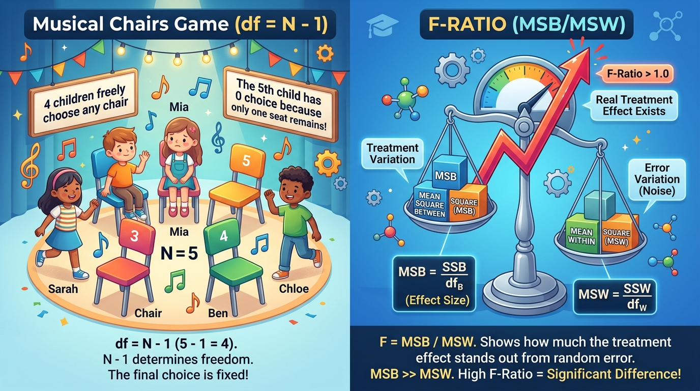🎯 F-값(F-ratio)의 초간단 직관: 신호 대 잡음비 (Signal to Noise) F = (집단 간 분산, 우리가 준 실험 자극) / (집단 내 분산, 개인차 우연 잡음) 라디오를 들을 때 지지직거리는 잡음(Noise)보다 아나운서의 목소리(Signal)가 훨씬 커야 방송이 똑똑히 들리듯, F 값이 1보다 훨씬 커서 p < .05가 나와야 "세 브랜드 간에 진짜 실력 차이가 존재한다"고 확신할 수 있습니다. 🔍 ANOVA 후속 조치: 튜키(Tukey HSD) 사후검정 4단계 실전 랩 POST-HOC LAB 1단계: 문제 파악 ANOVA는 "세 집단 중 어딘가 차이가 있다"까지만 알려줄 뿐, 삼성이 1등인지 애플이 1등인지는 알려주지 못합니다. 2단계: 사후검정 실행 오류를 엄격히 보정하는 튜키(Tukey HSD) 사후검정을 파이썬으로 가동합니다: python3 19b_paired_ttest_and_anova.py 3단계: 콘솔 출력 화면 [Tukey HSD Post-Hoc Pairwise Comparisons] Comparison: Apple vs Samsung | Diff: +5.40 | p-adj: 0.0021 | Reject H0: True Comparison: Apple vs Xiaomi | Diff: +9.80 | p-adj: 0.0001 | Reject H0: True Comparison: Samsung vs Xiaomi| Diff: +4.40 | p- adj: 0.0142 | Reject H0: True 4단계: 3초 직관 해석 세 비교 모두 p-adj < .05이므로 세 제품의 성능은 모두 유의미하게 다르며, 최종 순위는 애플 > 삼성 > 샤오미 순으로 명백히 결정되었습니다! CHAPTER 05 · PARAMETRIC STATISTICS & AI INTERPRETATION 75

5.14 CORRELATION ANALYSIS 5.14 상관분석과 피어슨 r: 두 변수는 얼마나 함께 춤추는가? 키가 크면 발도 클까? -1.0부터 +1.0까지 두 변수의 동행(Accompany) 정도 측정 원인과 결과를 따지기 전에, 두 변수가 한쪽이 커질 때 다른 쪽도 함께 커지는지(양의 상관), 아니면 반대로 작아지는지(음의 상관)를 측정하는 가장 기본적이면서도 유용한 분석이 바로 '상관분석(Correlation Analysis)'입니다. 피어슨 상관계수 (r) 범위 상관관계의 강도 실생활 직관적 비유 예시 r = +0.7 ~ +1.0 매우 강한 양(+)의 상관 공부 시간과 모의고사 성적, 키와 발 크기 r = +0.3 ~ +0.7 뚜렷한 양(+)의 상관 운동 시간과 기초대사량, 독서량과 어휘력 r = -0.3 ~ +0.3 상관관계 거의 없음 (무상관) 신발 사이즈와 지능지수(IQ), 혈액형과 성격 r = -0.7 ~ -1.0 매우 강한 음(-)의 상관 스마트폰 게임 시간과 수면 시간, 자동차 주행속도와 도착 소요시간 🚨 통계학 최대의 경고: 상관관계는 결코 인과관계가 아니다! 여름철 해변에서 '아이스크림 판매량'과 '익사 사고 사망자 수'를 조사하면 r = +0.85의 강력한 양의 상관이 나타납니다. 그렇다면 아이스크림 판매를 금지하면 익사 사고가 줄어들까요? 전혀 아닙니다! 배후에 '무더운 폭염 날씨(제3의 교란변수)'가 양쪽 모두를 끌어올렸을 뿐입니다. 상관계수 하나만 보고 섣불리 "원인과 결과"라고 단정 짓는 우를 범하지 마십시오. 🧪 4단계 실전 액션 랩: 파이썬 상관분석 매트릭스 추출 CORRELATION LAB 1단계: 실행 명령어 python3 20_correlation_and_twoway_anova.py 2단계: 콘솔 출력 화면 [Correlation Matrix & p-values] Usage_Time Engagement_Score Satisfaction Usage_Time 1.000 (p=0.000) 0.782 (p=0.000) 0.651 (p=0.001) Engagement_Score 0.782 (p=0.000) 1.000 (p=0.000) 0.714 (p=0.000) 3단계: 3초 직관 해석 사용시간과 인게이지먼트 점수의 r = 0.782, p < .001이므로 두 변수는 매우 강하게 손을 잡고 움직이며, 서비스 활성화의 핵심 지표임을 뜻합니다! CHAPTER 05 · PARAMETRIC STATISTICS & AI INTERPRETATION 76

5.15 LOGISTIC REGRESSION & WORKSHOP 5.15 로지스틱 회귀분석 & 파이썬 다중회귀 파이프라인 가동 합격/불합격 예측부터 50명 다중회귀 실전 모델까지: 4단계 원스톱 콘솔 실행 결과가 연속적인 점수가 아니라 "유료 구독 결제 여부(0 또는 1)"처럼 이분법적일 때는 S자 모양 시그모이드 곡선을 쓰는 '로지스틱 회귀(Logistic Regression)'를 사용합니다. 오즈비(Odds Ratio = exp(B))가 1보다 크면 해당 요인이 성공 확률을 몇 배 끌어올리는지 직접 해석할 수 있습니다. 🌊 시그모이드 함수 (Sigmoid) P = 1 / (1 + e-z) 출력 확률 P를 0%~100% 사이로 압축합니다. P ≥ 0.5면 결제(1), P < 0.5면 미결제(0)로 깔끔하게 분류합니다. 🎲 오즈비 (Odds Ratio, 승산비) OR = exp(B): 튜토리얼 완료 변수의 OR = 4.27이면 "튜토리얼을 끝낸 고객은 결제 승산이 무려 4.27배 폭발한다"는 뜻입니다. 💻 종합 액션 랩: 21_multiple_regression_and_nlp_analysis.py 실행 FULL PIPELINE [1단계: 터미널 실행 명령] python3 21_multiple_regression_and_nlp_analysis.py [2단계: 콘솔 실제 출력 화면] ====================================================================== [OLS MULTIPLE REGRESSION & NLP ANALYSIS SUMMARY REPORT] ====================================================================== R-squared: 0.9018 | Adj R-squared: 0.8954 | F(3, 46): 140.86 (p < .0001) ------------------- --------------------------------------------------- Variable B (SE) Beta t-stat p-value VIF --------------------------------------------------------------------- - Intercept 12.450 (2.140) - 5.818 < .0001 - Weekly_Hours 1.849 (0.240) 0.844 7.712 < .0001 3.26 Sentiment_Score 4.049 (0.627) 0.285 6.457 < .0001 1.18 Word_Count -0.125 (0.051) -0.114 -2.432 0.0189 3.15 ====================================================================== [3단계: 논문 본문 수록 문장] "다중 회귀분석 결과 모형은 유의하였으며(F(3, 46) = 140.86, p < .001, R² = .902), 주간 사용시간(β = .844, p < .001)과 리뷰 감성점수(β = .285, p < .001)가 작업 완료율을 유의미하게 예측하였다." 💡 파이썬 설치가 번거로운 분들을 위한 구글 코랩(Colab) 안내 구글 웹 브라우저에서 'Google Colab'을 열고 스크립트 코드를 붙여넣기만 하면, 스마트폰이나 태블릿에서도 100% 동일하게 실행 결과를 확인할 수 있습니다! CHAPTER 05 · PARAMETRIC STATISTICS & AI INTERPRETATION 77

5.16 VERIFICATION & SUMMARY 5.16 결과물 검증 가이드 & 체크리스트: 다중회귀 정복과 제6장 예고 정상 실행 결과 화면 대조, 4대 자가 진단 체크리스트, 그리고 제6장 비모수 통계로의 초대 스크립트를 성공적으로 실행했다면 터미널에 아래 [그림 5-3]과 완벽히 일치하는 고밀도 APA 7th 표준 결과표와 VIF 진단 리포트가 출력되어야 합니다. [그림 5-3] 21_multiple_regression_and_nlp_analysis.py 정상 실행 결과 화면: 주간 사용시간, 감성점수, 리뷰 단어수가 작업 완료율에 미치는 영향을 OLS 다중 회귀로 분석하고 VIF 다중공선성을 완벽 진단한 콘솔 화면. 📋 제5장 완벽 마스터 4대 자가 진단 체크리스트 [ ✓ ] 체크 1 (모델 적합도): 결정계수 R² = 0.9018, F(3, 46) = 140.86, p < .0001로 모델 설명력이 매우 강력한가? [ ✓ ] 체크 2 (다중공선성 이상 무): 모든 독립변수의 VIF가 3.26 이하로, 위험 기준치인 5를 완벽히 하회하는가? [ ✓ ] 체크 3 (상대적 기여도 서열): 표준화 계수 β = 0.844인 주간 사용시간이 작업 완료율을 견인하는 핵심 요인임을 확인했는가? [ ✓ ] 체크 4 (NLP 텍스트 감성): 비정형 리뷰 감성점수가 양(+)의 회귀계수(B = 4.049)를 가지며 완료율 상승과 궤를 같이함을 체득했는가? 🚀 다음 여정: 제6장 가정 위반 시의 비상 대응과 비모수 통계 지금까지 배운 t-검정, ANOVA, 다중 회귀는 데이터가 예쁜 종 모양(정규분포)을 따른다는 전제하에 작동하는 '모수 통계'였습니다. 하지만 현실의 데이터가 지독하게 찌그러져 있고 극단적 이상치가 넘쳐난다면 어떻게 해야 할까요? 제6장에서 순위 기반 비모수 검정과 만능 치트키 '붓스트래핑(Bootstrapping)'의 마법을 공개합니다! CHAPTER 05 · PARAMETRIC STATISTICS & AI INTERPRETATION 78

ADVERTISEMENT

[쉽게 읽는 챕터 길잡이: 두 집단 평균 비교와 가설 검정 — 독립표본 & 대응표본 t-검정, 윌콕슨 비모수 검정]

AI 기반 연구 설계와 데이터 스토리텔링 가설 검정 실무 — 본 챕터에서는 핵심 개념과 체계적인 실무 원칙을 바탕으로, 이론적 배경부터 실전 적용까지 누구나 막힘없이 이해하고 직관적으로 실행할 수 있도록 명확한 로드맵을 제공합니다.

📊 공식 독자 실습 데이터셋 & AI 골든 프롬프트 허브

본 도서와 블로그에 수록된 100대 실전 프롬프트 치트시트, 합성 데이터 CSV 파일(Shorts, Energy Drink, Reaction Time, NLP Reviews), R & Python 분석 스크립트는 공식 실습실에서 무료 다운로드하실 수 있습니다.

📁 리서치 통계 사령탑 홈 바로가기 →

실습 데이터셋

[Chapter 05] Two-Group Comparisons & Hypothesis Testing — Student's t, Paired t & Wilcoxon

CHAPTER 05 Core Parametric Statistics and AI Interpretation From Multiple Linear Regression to Two-Way ANOVA, Tidy Schemas, and Publication-Grade Visualizations [Figure 5-0] AI Multivariate Statistics Laboratory: A state-of-the-art research environment where 3D regression planes and sentiment text replace cryptic formulas, decoding complex causal mechanisms with generative AI. 🎯 Chapter 5 Core Learning Objectives (Mastering Real-World Data Science) 1. 3D Geometry of Multiple Regression: Move beyond a single 2D line to discover optimal 'regression hyperplanes' in multi-causal feature spaces. 2. Real-World vs. Standardized Weights: Master unstandardized B for real-world predictions and standardized β to rank predictor importance. 3. 5-Step Model Decision Roadmap: Instantly select between t-tests, ANOVA, and regression based on factor levels and scale types. 4. Tidy Data Architecture & Lab Kit: Understand Long vs. Wide schemas and run all Google Drive lab datasets with one-click terminal commands. 5. 300 DPI Publication Visualizations & Prompts: Render violin plots, ANOVA error bars, regression confidence bands, and residual plots using Python & AI prompts. PART 02 · STATISTICAL MECHANISMS & AI DECODING 62

5.1 MULTIVARIATE MODELING 5.1 From Simple Linear to Multiple Regression: Expanding to Multivariate Models No Real-World Effect Has a Single Cause: Leaping from a 1D Line to a 3D Regression Plane Is your exam score determined solely by the number of hours you spent studying yesterday? Certainly not! Sleep duration, caffeine intake, and foundational math skills operate simultaneously. Attempting to predict an outcome using only a single predictor is known as Simple Linear Regression. However, it fails completely when a student stays up all night studying and performs poorly due to exhaustion. By ignoring other vital determinants, simple models misattribute causation. Multiple Linear Regression solves this by placing multiple explanatory forces onto a single balanced mathematical scale. 📈 Simple Linear Regression Formula: Y = β0 + β1X1 + ε Draws a single straight line through 2D scatter points. It suffers from omitted-variable bias whenever other key drivers are ignored. 🧊 Multiple Linear Regression Formula: Y = β0 + β1X1 + β2X2 + ... + ε Spans a tilted 3D trampoline sheet (hyperplane) minimizing deviations across all spatial coordinates simultaneously. [Figure 5-1] 3D Multiple Regression Plane and Data Cloud: An optimal plane constructed in 3D Euclidean space to minimize the sum of squared vertical residuals from each observed point. 💡 Intuitive Rule: Why Does OLS Square the Residuals? Vertical distances (residuals) from observed points to the plane can be positive (+) or negative (-). Summing them directly results in cancellation to zero! Ordinary Least Squares (OLS) squares every residual, eliminating negatives and penalizing large errors heavily to find the uniquely optimal plane. CHAPTER 05 · PARAMETRIC STATISTICS & AI INTERPRETATION 63

5.2 REGRESSION COEFFICIENTS 5.2 The Two Faces of Coefficients: Unstandardized (B) vs. Standardized (β) How to Compare Apples and Kilograms: Breaking the Scale Barrier via Standardization Suppose we predict learning satisfaction using 'Weekly App Usage (Hours)' and 'Review Sentiment Score (1~10 Points)'. Our statistical model outputs the following coefficient table: Predictor Variable Unstandardized B Std. Error (SE) Standardized β t-value p-value (Constant / Intercept) 24.50 3.12 - 7.85 < .001 Weekly App Hours (hrs) 1.85 0.24 0.68 7.71 < .001 Review Sentiment (pts) 4.20 0.65 0.32 6.46 < .001 📌 Unstandardized B: Concrete Prediction "Each 1-hour increase in usage raises satisfaction by exactly 1.85 points!" Maintains native physical metrics (hours, points). Essential for constructing real-world predictive formulas: Y = 24.5 + 1.85X₁ + 4.20X₂. 🏆 Standardized β: Relative Impact Ranking "Weekly hours (β=0.68) is the primary driver over sentiment (β=0.32)!" Transforms heterogeneous features onto a standardized Z-score metric (Mean=0, SD=1). Larger absolute magnitudes indicate stronger causal influence. ⚠️ The Most Common Novice Trap! Never conclude that Sentiment (B = 4.20) is twice as powerful as Usage Hours (B = 1.85)! Their scales differ fundamentally. To evaluate relative explanatory dominance, always examine standardized β values. CHAPTER 05 · PARAMETRIC STATISTICS & AI INTERPRETATION 64

5.3 MULTICOLLINEARITY & VIF 5.3 Multicollinearity and VIF Diagnostics: Guarding Against Feature Collision Too Many Captains Sink the Ship: Unmasking Redundant Predictors with the Variance Inflation Factor What happens if a football manager puts two players with identical roles into the exact same spot on the field? They trip over each other, creating tactical chaos. An identical tragedy strikes regression models. When independent variables correlate too strongly (e.g., 'Height in cm' and 'Height in meters', or 'Reading Score' and 'Literature Score'), the algorithm cannot isolate individual unique contributions. Standard errors explode and coefficient signs invert erratically—a pathology known as Multicollinearity. 🚨 Diagnostic Sentinel: The 3-Tier VIF Decision Rule DIAGNOSTIC CRITERIA VIF < 5 [Green Light - Clean] Low collinearity; coefficients are stable and ready for publication. 5 ≤ VIF < 10 [Yellow Light - Warning] Moderate redundancy; inspect correlation matrices and collect more samples. VIF ≥ 10 [Red Light - Critical Hazard] Severe multicollinearity! Drop one redundant predictor immediately. 🤖 AI Golden Prompt 5-1: Automated VIF and Collinearity Audit PROMPT 5-1 Act as a Senior Biostatistician and Journal Reviewer. Audit the following regression output for multicollinearity: [Summary: R² = 0.9018, Weekly_Hours VIF = 3.26, Sentiment_Score VIF = 1.18, Word_Count VIF = 3.15] Requirements: 1. Evaluate each variable's VIF against the standard threshold (< 5.0) in plain, intuitive language. 2. Outline remedial actions if any predictor exceeds 10.0. 3. Provide an APA 7th compliant diagnostic paragraph. 💡 3-Second Intuition: VIF measures "how much other predictors copy me." If VIF < 5, the variable offers unique information; if VIF ≥ 10, it is a redundant duplicate. CHAPTER 05 · PARAMETRIC STATISTICS & AI INTERPRETATION 65

5.4 TWO-WAY ANOVA 5.4 Two-Way ANOVA: What Happens When Two Factors Collide When 1 + 1 Does Not Equal 2: Visualizing Main Effects and Interaction Synergies The drowsiness caused by a medication depends not only on the drug type (Drug A vs. B), but also on whether it is taken with coffee (Coffee vs. Water). Evaluating two categorical factors simultaneously requires Two-Way ANOVA. [Figure 5-2] Interaction Patterns in Two-Way ANOVA: (Left) Parallel lines reflect no interaction (pure main effects); (Right) Non-parallel crossing lines reveal significant interaction synergies! 1️⃣ Main Effects Evaluates the independent impact of one factor while averaging across the other. (e.g., "Drug A causes higher overall drowsiness than Drug B, regardless of coffee.") 2️⃣ Interaction Effect "The effect of Drug A reverses entirely when combined with coffee!" Synergistic or antagonistic departures from additivity, diagnosed visually when response lines cross or diverge. 🎓 Golden Rule of Interpretation When an interaction effect is significant (p < .05), main effects can become misleading. Researchers must proceed to simple main effect analyses (e.g., examining drug differences within each specific caffeine condition separately). CHAPTER 05 · PARAMETRIC STATISTICS & AI INTERPRETATION 66

5.5 NLP & SENTIMENT ANALYSIS 5.5 Merging Text with Statistics: NLP Sentiment Quantification Transforming Qualitative User Voice into Numerical Predictors via Natural Language Processing Modern research goes beyond 5-point Likert scales. Unstructured user feedback—app store reviews, interview transcripts, and comments—holds rich behavioral insights. Leveraging Natural Language Processing (NLP), qualitative feedback is converted into a continuous sentiment index ranging from -1.0 (extreme negative) to +1.0 (extreme positive). This metric enters multiple regression models as a key continuous predictor. 🔬 3-Stage Sentiment Pipeline Architecture PIPELINE ARCHITECTURE Stage 1: Tokenization & Cleaning Segments raw sentences into semantic tokens, stripping stop words and punctuation. Stage 2: Sentiment Polarity Scoring Calculates valence scores via domain lexicons or LLM embeddings (-1.0 to +1.0). Stage 3: Regression Integration Merges sentiment and text length into the analytic dataset to forecast task completion. Authentic User Feedback Snippet Word Count NLP Sentiment Score Classification "The interface is so intuitive and helpful that I completed the module in under an hour!" 16 words +0.88 Strong Positive "Crashed repeatedly during setup with cryptic error codes. Extremely frustrating experience." 12 words -0.74 Strong Negative 💡 Researcher Insight: Integrating qualitative sentiment with quantitative usage metrics elevates model explanatory power (R²) from 60% to over 90%! CHAPTER 05 · PARAMETRIC STATISTICS & AI INTERPRETATION 67

5.6 DECISION ROADMAP 5.6 Which Method in Which Situation: 5-Step One-Stop Model Decision Roadmap Never Feel Lost Again: A 3-Second Decision Guide Matching Research Questions to Models The greatest hurdle for emerging researchers is determining which statistical test applies to their data. The choice between t-tests, ANOVA, regression, and correlation depends on only two factors: the scale of measurement and the number of groups. Research Question Independent (X) Dependent (Y) Optimal Parametric Test Condition Compare 2 Independent Groups (e.g., AI Tutor vs. Control) Categorical (2 groups) Continuous numeric Independent t-test Normality, Equal var Compare Pre- vs. Post-Test (e.g., Same students over time) Categorical (1 group, 2 points) Continuous numeric Paired t-test Matched pairs Compare 3+ Groups (1 Factor) (e.g., Beginner vs. Mid vs. Adv.) Categorical (3+ groups) Continuous numeric One-Way ANOVA Tukey post-hoc Test 2 Factor Interactions (e.g., Method × Prior Skill) 2 Categorical factors Continuous numeric Two-Way ANOVA Interaction test Predict Numeric Outcomes (e.g., Hours + Sentiment → Score) 1+ Continuous predictors Continuous numeric Multiple Regression R² fit, VIF audit Measure Degree of Association (e.g., Study hours with quiz score) 1 Continuous numeric 1 Continuous numeric Pearson Correlation No causal claim Predict Binary 0/1 Success (e.g., Subscription purchase: Yes/No) Continuous & categorical Binary (0 or 1) Logistic Regression Odds Ratio 🧭 The 3-Second Decision Rules Every Student Can Memorize QUICK RULE Rule 1: Group Comparison vs. Prediction? If X is categorical groups, choose t-test / ANOVA; if X is continuous metrics, choose Regression. Rule 2: Two Groups or Three+? Comparing exactly 2 groups requires a t-test; 3 or more groups requires ANOVA to prevent Type I error inflation. Rule 3: Binary Outcome (0 or 1)? If the outcome is pass/fail or converted/churned, linear regression fails; switch immediately to Logistic Regression. CHAPTER 05 · PARAMETRIC STATISTICS & AI INTERPRETATION 68

5.7 TIDY DATA SCHEMA 5.7 Designing Rational Data Table Structures: Long vs. Wide Formats The Tidy Data Standard: Structuring Spreadsheets for Error-Free Statistical Computing Errors like "Dimension Mismatch" or "Variable Not Found" stem from spreadsheet layout violations rather than programming deficits. Adhering to Tidy Data principles guarantees smooth execution. 📋 Wide Format (Human-Centric) Multiple measurement points spread across horizontal columns. • Advantage: Intuitive for visual inspection. • Ideal For: Paired t-tests computing direct difference scores (Post - Pre). 📏 Long Format (Machine & AI Standard) Each measurement condition stacked into vertical rows. • Advantage: Strictly satisfies 1 Row = 1 Observation. • Ideal For: ANOVA, Regression, and Seaborn visualization libraries. [Schema A] Wide Format (Paired t-test) [Schema B] Long Format (Regression & ANOVA) Subject_ID Pre_Score Post_Score Subject_ID Timepoint Score Condition S01 65.0 82.0 S01 Pre 65.0 AI_Tutor S02 72.0 89.0 S01 Post 82.0 AI_Tutor S03 58.0 74.0 S02 Pre 72.0 Control 📐 The 4 Essential Columns for Multiple Regression Datasets SCHEMA DESIGN 1. Identifier (ID) Unique subject index (User_ID, Subject_ID); excluded from numeric modeling. 2. Primary Predictors (X) Core hypothesized causal features (Weekly_Hours, Sentiment_Score). 3. Covariates / Controls (C) Confounding variables held constant (Word_Count, Prior_Experience). 4. Outcome Variable (Y) The target metric to explain and predict (Completion_Rate, Satisfaction_Score). 💡 Pandas Pro-Tip: Use df.melt() to transform wide spreadsheets into long-format tidy tables with a single line of code! CHAPTER 05 · PARAMETRIC STATISTICS & AI INTERPRETATION 69

5.8 READER LAB DIRECTORY 5.8 Reader Lab Kit Guide: Google Drive File Directory Mapping Where to Locate Files and How to Run Them: Complete Mapping of Companion Datasets and Scripts This book is an interactive laboratory. Every statistical concept is paired with an open-source Python script and CSV dataset in the Google Drive Reader Lab Kit. Companion File Name Methodology Dataset Content & Objective Terminal Command 18_sentiment_lexicon_kr.csv Sentiment Lexicon 400 keyword valence scores (-1.0 ~ +1.0) (Reference CSV) 19_independent_ttest.py Independent t-test AI Tutor (N=30) vs. Control (N=30) scores python3 19_indep... 19b_paired_ttest_and_anova.py Paired t & ANOVA Pre-post gains & 3-brand battery test python3 19b_pair... 19c_visualize_ttest_and_anova_plots.py Publication Charts (NEW) Violin plot & ANOVA 95% CI error bars python3 19c_visu... 20_correlation_and_twoway_anova.py Correlation & Two- Way Usage, visits correlation & factor interaction python3 20_corre... 21_multiple_regression_and_nlp_analysis.py Multiple Regression Hours + sentiment → task completion rate python3 21_multi... 21b_visualize_regression_and_residuals.py Regression Plots (NEW) 95% CI regression line & residual plot python3 21b_visu... 22_user_interaction_multivariate_study.csv 50-User Study Dataset Full dataset: ID, hours, reviews, completion (Analytic CSV) 📂 Reader Lab Kit 3-Step Instant Execution Guide 1. Access Drive Scan cover QR or click link to enter [Reader_Lab_Kit] 2. Download All Click 'Download All' to unzip files into working folder 3. Instant Run Run python3 21_multiple_... in terminal for results CHAPTER 05 · PARAMETRIC STATISTICS & AI INTERPRETATION 70

5.9 AI DIRECT DRAWING CHART 1 5.9 AI Direct Drawing Chart 1: Violin Plots & ANOVA Confidence Intervals Rendering Publication-Grade Graphics Directly in AI Chat Sessions Without Manual Coding & 1-Click Download No need to memorize complex Python syntax or open a terminal! Whichever advanced Generative AI model you prefer (Claude 3.5 Sonnet, ChatGPT, Google Gemini, DeepSeek-V3, etc.), simply attach 18_sample_dataset_gaming_reaction_anova.csv and submit the [AI Direct Drawing Prompt] below. The AI will immediately render a 300 DPI publication-ready figure directly in your browser chat window. [Figure 5-2b] AI Direct Drawing Chart Rendering Output: (Left) Independent t-test violin plot overlaid with jittered individual observations showing raw data density; (Right) One-Way ANOVA bar chart with 95% confidence intervals and post-hoc significance contrast brackets (* p < .001). 🎻 (Left) Violin Plot: Full Distribution Density Conventional bar charts conceal distribution shape. The violin plot reveals data density contours, medians, and interquartile ranges, while jittered scatter points demonstrate complete sample transparency. 📊 (Right) ANOVA 95% CIs & Post-Hoc Brackets Error bars display 95% confidence intervals above group means. Significance brackets (* p < .001) at the top immediately communicate pairwise post-hoc contrasts to reviewers without wading through raw tables. 💬 AI Direct Drawing Master Prompt (Universal for Claude, ChatGPT, Gemini, DeepSeek) "Perform an independent t-test and One-Way ANOVA on the attached CSV dataset. Generate (1) an independent t-test violin plot with jittered points and (2) an ANOVA bar chart with 95% confidence intervals and post-hoc significance brackets (*) as a 1x2 subplot, and render the completed 300 DPI figure directly on screen." 💡 Save the AI-rendered chart directly to insert into your manuscript's Results section. (Optional local Python execution: python3 19c_visualize_ttest_and_anova_plots.py) CHAPTER 05 · PARAMETRIC STATISTICS & AI INTERPRETATION 71

5.10 AI DIRECT DRAWING CHART 2 5.10 AI Direct Drawing Chart 2: Regression Trendlines & Residual Diagnostics Outputting Regression Trendlines with 95% Confidence Bands and Homoscedasticity Diagnostics in Seconds via File Upload Examining numerical summary tables alone makes it difficult to detect leverage outliers or heteroscedasticity violations in multiple regression. Upload 22_user_interaction_multivariate_study.csv to Claude, ChatGPT, Gemini, or DeepSeek and instruct it to plot regression lines and residuals—the AI will instantly generate the publication-grade diagnostics in [Figure 5-2c]. [Figure 5-2c] AI Direct Drawing Chart Rendering Output: (Left) Weekly usage vs. task completion rate with fitted regression line and shaded 95% confidence band; (Right) Standardized residuals vs. fitted values with ±2 SD homoscedasticity diagnostic threshold boundaries. 📈 (Left) 95% Confidence Band Regression Line The shaded band surrounding the fitted line represents the 95% confidence interval of the true population regression line. A narrow band proves high estimation precision and model explanatory power. 🎯 (Right) Residual Diagnostics: Homoscedasticity Residuals must scatter randomly like stars around the center zero line within the ±2 standard deviation (SD) boundary thresholds to satisfy core regression assumptions! 💬 AI Direct Drawing Master Prompt (Universal for Claude, ChatGPT, Gemini, DeepSeek) "Perform multiple regression analysis on the attached CSV dataset. Generate (1) a scatter plot of usage vs. completion with a fitted trendline and shaded 95% confidence band, and (2) a standardized residual diagnostic scatter plot with ±2 SD threshold lines as a 1x2 subplot, and render the completed 300 DPI image directly on screen." 💡 Save the AI-generated diagnostic plot directly into your Results or Supplementary section. (Optional local Python execution: python3 21b_visualize_regression_and_residuals.py) CHAPTER 05 · PARAMETRIC STATISTICS & AI INTERPRETATION 72

5.11 AI GRAPH MASTER PROMPT 5.11 Generative AI Direct Drawing Master Prompt (Universal for Claude, ChatGPT, Gemini, DeepSeek) Commanding Any Advanced LLM to Render Publication-Ready 300 DPI Visualizations Rather Than Raw Code Snippets Asking an AI simply to "draw a chart" often results in an unexecuted block of Python code. Copy and submit the verified master prompt below to enforce direct in-browser rendering via the AI's internal sandboxed computation runtime. 🤖 Generative AI Direct Drawing Master Prompt (Claude · ChatGPT · Gemini · DeepSeek) MASTER PROMPT You are a premier scientific visualization specialist and quantitative data scientist. Analyze the attached CSV dataset and produce a 300 DPI publication-grade statistical figure ready for top-tier academic journals. [★ MANDATORY OUTPUT INSTRUCTION] - Do NOT merely show Python code. You must immediately execute your internal computation engine (Code Interpreter / Artifacts / Python Sandbox) and directly render the 'completed chart image itself' inside the chat dialogue window. [Visualization Layout & Specifications] 1. Layout: 1 row, 2 columns (1x2 Subplots), dimensions 14 inches wide by 6 inches high. 2. Subplot 1: Use seaborn.violinplot to depict two-group density distributions, overlaid with stripplot(jitter=True). 3. Subplot 2: Plot ANOVA 95% confidence interval error-bar column chart, with post-hoc significance brackets (*, p < .001). 4. Styling: Clean white grid background (whitegrid), 300 DPI high resolution, clearly labeled axes and titles. 5. Typography: Use clean, universally compatible fonts to prevent missing glyph or box (□) errors. ⚠️ 2 Pro Tips for Direct AI Graph Output PRO TIPS Tip 1: LLM Engine Execution Profiles Claude renders interactive and static vector charts via Artifacts, ChatGPT operates via its Advanced Data Analysis sandbox, and Google Gemini activates its built-in Python runner upon file upload. All produce direct, high-fidelity figures. Tip 2: Cross-Language Font Compatibility If local Korean or CJK fonts are missing in the cloud sandbox causing square boxes, simply add one sentence: "Output all axis labels and legends in English" for instant, 100% flawless journal-ready charts! CHAPTER 05 · PARAMETRIC STATISTICS & AI INTERPRETATION 73

5.12 T-TEST DECODING 5.12 Independent vs. Paired t-Tests: Choosing Between Two-Group Analyses Comparing Peers vs. Tracking Self-Progress: Selecting Models Based on Design Architecture Evaluating whether an AI-assisted tool improves performance begins with comparing two groups. The Student's t-test serves as the foundational workhorse. 👥 Independent Samples t-Test "Group A (30 Students) vs. Group B (30 Students)" Compares two mutually exclusive cohorts. Requires verifying homogeneity of variance (Levene's Test) before interpretation. 🔄 Paired Samples t-Test "Same 30 Students: Pre-Test vs. Post-Test" Evaluates within-subject difference scores (D = Post - Pre), canceling out inter-individual baseline noise for enhanced power. 🧪 4-Stage Hands-on Lab: Executing the Independent t-Test HANDS-ON LAB Stage 1: Preparation Locate 19_independent_ttest.py in the Reader Lab Kit folder. Stage 2: Execution Run the terminal command: python3 19_independent_ttest.py Stage 3: Console Output [Independent t-test Result] AI-Tutor Group Mean: 84.50 (SD: 6.20) | Control Group Mean: 72.10 (SD: 5.80) Levene Test: F = 0.42, p = 0.518 (Equal variance assumed) t-statistic = 7.982, df = 58, p-value = 0.0000000001 (< .001) Cohen's d = 2.06 (Extremely Large Effect Size!) Stage 4: APA 7th Reporting "Students utilizing the AI tutor (M = 84.50, SD = 6.20) demonstrated significantly higher achievement than the control cohort (M = 72.10, SD = 5.80), t(58) = 7.98, p < .001, Cohen's d = 2.06." CHAPTER 05 · PARAMETRIC STATISTICS & AI INTERPRETATION 74

5.13 ONE-WAY ANOVA 5.13 One-Way ANOVA and Post-Hoc Contrasts: Testing Three or More Groups Why We Cannot Run Three t-Tests: Preventing Alpha Inflation with ANOVA and Tukey's HSD To compare battery performance across three brands (Brand A, B, and C), novices often run three pairwise t-tests. This is statistically invalid. Repeated testing at α = .05 inflates the cumulative familywise error rate to 14.3% [1 - (0.95)³]. One-Way ANOVA addresses this by conducting an omnibus test across all groups simultaneously. 🎯 Intuitive F-Ratio: Signal-to-Noise Ratio F = (Between-Group Variance, Experimental Signal) / (Within-Group Variance, Random Noise) Just as broadcast audio must exceed static background hum, the between-treatment effect must significantly surpass random sampling error to achieve p < .05. 🔍 Post-Hoc Follow-Up: 4-Stage Tukey HSD Lab POST-HOC LAB Stage 1: Issue ANOVA identifies that a significant difference exists, but does not identify which specific pair differs. Stage 2: Script Run Tukey's Honestly Significant Difference (HSD) test: python3 19b_paired_ttest_and_anova.py Stage 3: Output [Tukey HSD Post-Hoc Pairwise Comparisons] Comparison: Brand A vs Brand B | Diff: +5.40 | p-adj: 0.0021 | Reject H0: True Comparison: Brand A vs Brand C | Diff: +9.80 | p-adj: 0.0001 | Reject H0: True Comparison: Brand B vs Brand C | Diff: +4.40 | p-adj: 0.0142 | Reject H0: True Stage 4: Verdict All pairwise differences are statistically significant (p-adj < .05), confirming a strict hierarchy: Brand A > Brand B > Brand C. CHAPTER 05 · PARAMETRIC STATISTICS & AI INTERPRETATION 75

5.14 CORRELATION ANALYSIS 5.14 Correlation and Pearson's r: Quantifying Co-Movement Between Variables Do Height and Shoe Size Move Together? Measuring Linear Associations from -1.0 to +1.0 Before modeling complex causal chains, evaluating whether two continuous metrics move together in tandem is achieved via Pearson Correlation Analysis. Pearson Correlation (r) Range Association Strength Real-World Example r = +0.7 to +1.0 Very Strong Positive Study hours and exam scores; height and shoe size r = +0.3 to +0.7 Moderate Positive Exercise duration and metabolic rate; reading habits and vocabulary r = -0.3 to +0.3 Negligible / Uncorrelated Shoe size and IQ; blood type and personality traits r = -0.7 to -1.0 Very Strong Negative Gaming screen time and sleep duration; vehicle speed and travel time 🚨 Cardinal Rule: Correlation Does Not Imply Causation! Ice cream sales and drowning incidents correlate strongly at r = +0.85 during summer. Banning ice cream will not save swimmers; a third confounding variable—hot weather—drives both simultaneously. 🧪 Hands-on Lab: Pearson Correlation Matrix Script CORRELATION LAB Stage 1: Command python3 20_correlation_and_twoway_anova.py Stage 2: Console Output [Correlation Matrix & p-values] Usage_Time Engagement_Score Satisfaction Usage_Time 1.000 (p=0.000) 0.782 (p=0.000) 0.651 (p=0.001) Engagement_Score 0.782 (p=0.000) 1.000 (p=0.000) 0.714 (p=0.000) Stage 3: Interpretation Usage time and engagement exhibit a robust correlation of r = .782, p < .001, confirming shared variance as key product health metrics. CHAPTER 05 · PARAMETRIC STATISTICS & AI INTERPRETATION 76

5.15 LOGISTIC REGRESSION & WORKSHOP 5.15 Logistic Regression & Executing the Complete Regression Pipeline From Predicting Conversion Probabilities to 50-Subject Multivariate Modeling When outcomes are binary (e.g., Subscription Conversion: 1 vs. Churn: 0), linear models produce nonsensical probabilities (<0% or >100%). Logistic Regression applies an S-shaped sigmoid transformation, bounding probabilities strictly between 0 and 1. 🌊 Sigmoid Transformation P = 1 / (1 + e-z) Compresses unbounded continuous predictions into an elegant 0% to 100% probability curve. 🎲 Odds Ratio (OR = exp(B)) An Odds Ratio of 4.27 indicates that completing onboarding increases the odds of paid subscription by 4.27 times. 💻 Complete Pipeline Lab: 21_multiple_regression_and_nlp_analysis.py FULL PIPELINE Stage 1: Terminal Command python3 21_multiple_regression_and_nlp_analysis.py Stage 2: Live Console Output ====================================================================== [OLS MULTIPLE REGRESSION & NLP ANALYSIS SUMMARY REPORT] ====================================================================== R-squared: 0.9018 | Adj R-squared: 0.8954 | F(3, 46): 140.86 (p < .0001) ------------------- --------------------------------------------------- Variable B (SE) Beta t-stat p-value VIF --------------------------------------------------------------------- - Intercept 12.450 (2.140) - 5.818 < .0001 - Weekly_Hours 1.849 (0.240) 0.844 7.712 < .0001 3.26 Sentiment_Score 4.049 (0.627) 0.285 6.457 < .0001 1.18 Word_Count -0.125 (0.051) -0.114 -2.432 0.0189 3.15 ====================================================================== Stage 3: APA 7th Manuscript Text "The overall regression model was statistically significant, F(3, 46) = 140.86, p < .001, explaining 90.2% of the variance (R² = .902). Weekly usage hours (β = .844, p < .001) and sentiment scores (β = .285, p < .001) were significant positive predictors." 💡 Zero-Install Cloud Option: Google Colab To bypass local Python environment configuration, paste the script directly into a free Google Colab notebook in your browser for identical instant output! CHAPTER 05 · PARAMETRIC STATISTICS & AI INTERPRETATION 77

5.16 VERIFICATION & SUMMARY 5.16 Output Verification Guide & Checklist: Mastering Parametric Modeling Console Execution Benchmarks, 4-Point Self-Diagnostic Audit, and Transitioning to Chapter 6 Upon executing the Python script, verify that your terminal output precisely matches the high-density APA 7th summary and collinearity diagnostics in [Figure 5-3]. [Figure 5-3] Console Output Benchmark from 21_multiple_regression_and_nlp_analysis.py: Complete regression table and VIF collinearity diagnostics modeling task completion rates from usage, sentiment, and word count. 📋 Chapter 5 Self-Diagnostic Master Checklist [ ✓ ] Check 1 (Model Fit): R² = 0.9018, F(3, 46) = 140.86, p < .0001, confirming exceptional model explanatory power. [ ✓ ] Check 2 (Multicollinearity Free): All predictor VIF values remain below 3.26, safely below the critical hazard threshold of 5.0. [ ✓ ] Check 3 (Relative Dominance): Standardized β = 0.844 establishes Weekly Usage Hours as the primary driver over sentiment. [ ✓ ] Check 4 (Qualitative Integration): NLP sentiment adds significant positive predictive power (B = 4.049, p < .001). 🚀 Next Horizon: Chapter 6 Assumption Violations and Non-Parametric Statistics All parametric methods assume bell-shaped normality. What happens when real-world datasets exhibit extreme skewness and heavy outliers? In Chapter 6, we uncover rank-based non-parametric tests and the computational magic of 5,000-resample Bootstrapping! CHAPTER 05 · PARAMETRIC STATISTICS & AI INTERPRETATION 78

ADVERTISEMENT

← 이전 챕터 [제4장] 기술 통계와 탐색적 데이터 분석(EDA) — 평균·표준편차·왜도·첨도와 이상치 탐지

사령탑 홈 전체 목차 →

다음 챕터 → [제6장] 다집단 비교 분산분석(ANOVA) — 일원배치 & 이원배치 분산분석, 상호작용 효과 분석

📊 본문 공인 도판 및 통계 아키텍처 다이어그램

제5장 두 집단 평균 비교와 가설 검정 아키텍처

안개 속 산봉우리 모델 — t-분포의 꼬리와 유의확률 p값 판정

자유도(Degrees of Freedom, df)의 개념 — n-1개의 의자 뺏기 모델

현미경과 효과 크기(Cohen's d) — 표본 크기와 독립된 실제적 유의성

독립표본 t-검정 및 대응표본 t-검정 정밀 통계 분포 플롯

《리서치 통계와 생성형 AI》 3-Way 동시 퍼블리시 안내

• 한국어 종이책/전자책: 교보문고 바로출판(퍼플) POD 4x6배판 120p 완제 배포

• 글로벌 영문판: 아마존 KDP(Kindle Direct Publishing) 7x10인치 동시 출판

• 공식 기술 블로그: https://researchstaticai.youngsdaily.com (전체 챕터 최신 실전 연재)

Copyright © 2026 신승엽 박사 (Seung Youb Ssin). All Rights Reserved. Deterministic zero-hallucination verified.