[제3장] 실험실 캘리브레이션과 합성 데이터 시뮬레이션 — 하드웨어 지연 제어와 직사각형 Tidy Data

🇰🇷 한국어 정규 에디션 (교보문고 바로출판 POD 120p 완제 원문)

2.8 LAB CALIBRATION & DATA STRUCTURE 2.8 실전 연구소 프로토콜 1: 리서치 스트럭처와 실험 장비·환경 캘리브레이션 가설의 조작적 정의부터 모니터 주사율, 입력 장치 폴링 레이트, 방음·조도 통제 및 원시 로그 Tidy화 통계 교과서는 "두 집단의 반응시간을 측정했다"는 한 줄로 실험을 요약하지만, 실제 연구 현장에서는 하드웨어의 수십 밀리초(ms) 지연과 통제되지 않은 조명·소음이 처치 효과를 완전히 집어삼킵니다. 독립변수의 인과적 효과를 순수하게 추출하기 위해서는 실험 장비와 물리적 환경을 완벽하게 캘리브레이션하고, 수집되는 모든 시계열 로그를 통계 분석용 직사각형 Tidy Data로 자동 정렬하는 리서치 파이프라인을 사전에 구축해야 합니다. ⚙️ 실험실 핵심 하드웨어 3대 정밀 캘리브레이션 (System Latency Control) 디스플레이 주사율 (Refresh Rate) 일반 60Hz 모니터는 프레임당 16.67ms 지연이 발생합니다. 인지 반응 실험은 반드시 144Hz(6.94ms) 또는 240Hz(4.17ms) 고주사율 모니터로 통일하여 자극 제시 시차 오차를 5ms 이내로 억제해야 합니다. 입력 장치 폴링 레이트 (Polling Rate) 사무용 마우스(125Hz)는 신호 입력에 최대 8ms의 지연이 누적됩니다. 게이밍 기어급 1000Hz(1ms 주기 보고) 마우스/기계식 키보드를 표준 장비로 고정하여 입력 버퍼 잡음을 원천 차단합니다. 타임스탬프 하드웨어 동기화 자극이 화면에 표시되는 순간(V-Sync)과 피험자의 키 입력 시점을 파이썬 time.perf_counter_ns() 고해상도 타이머로 동기화하여 밀리초 미만의 정밀도를 보장합니다. 🏛️ 물리적 환경 통제 (Environmental Rigor) • 조도(Lux) 표준화: 실험실 조도를 300~500 Lux로 일정하게 유지(암막 커튼 및 LED 고정 광원 사용, 일조 변화 차단). • 음향 차음(Acoustic Isolation): 주변 소음 30 dB 이하 유지 또는 모든 피험자에게 동일한 액티브 노이즈 캔슬링(ANC) 헤드폰 착용 의무화. • 시야 거리 및 체위: 턱 받침대(Chin-rest) 또는 60cm 모니터 거리 고정으로 시야각(Visual Angle) 일관성 확보. 📋 원시 로그 → Tidy Data 스키마 매핑 실험 프로그램(PsychoPy/파이썬)이 기록하는 원시 타임스탬프 로그는 제3장에서 다룰 직사각형 롱 포맷(Long-Format Tidy Data)으로 자동 변환됩니다: Subject_ID | Group | Block | Trial | Reaction_Time | Accuracy 이 단일 행(Row) 단위 구조가 갖춰져야 제4장의 t-검정, ANOVA, 제5장의 회귀분석으로 직결됩니다! 💡 연구 현장 원포인트 레슨: "잡음을 줄이면 필요한 피험자 수가 절반으로 줄어든다" 하드웨어 딜레이와 환경 잡음(σ²_error)을 방치하면 분모(잡음)가 커져 t-값과 F-비가 깎여나갑니다. 조도와 모니터 주사율을 철저히 캘리브레이션하여 측정 분산을 20% 줄이는 것은, 피험자 30명을 추가로 모집하는 것보다 통계적 검정력을 올리는 데 훨씬 경제적이고 강력합니다! CHAPTER 02 · EXPERIMENTAL DESIGN & SUBJECT ALLOCATION 26

2.9 PARTICIPANT LOGISTICS & LAB SOP 2.9 실전 연구소 프로토콜 2: 피험자 로지스틱스와 실험 실행 표준운영절차(SOP) G*Power 검정력 기반 N수 산정, 15% 탈락 버퍼, 라틴방격 타임 슬롯 및 5단계 완결 SOP 실험실 현장에서 가장 뼈아픈 실수는 "피험자 몇 명을 모아서 어떤 순서로 돌릴 것인가?"에 대한 정밀한 계획 부재에서 터져 나옵니다. 표본 크기가 부족하면 참된 효과를 발견하지 못하는 제2종 오류(β)에 빠지고, 피험자들의 시간대와 컨디션을 통제하지 못하면 생체 리듬 (Circadian Rhythms) 교란 요인이 처치 효과로 둔갑합니다. 검증된 과학적 로지스틱스와 엄격한 SOP를 준수해야 합니다. 📊 피험자 N수 산정 공식과 15% 탈락 안전 버퍼(Safety Buffer) 법칙 • 선험적 검정력 분석(A Priori Power Analysis): 학술 표준 검정력 1 - β = 0.80, 유의수준 α = 0.05, 중간 효과 크기(Cohen's d = 0.50) 기준, 독립표본 t-검정에 필요한 이론적 최소 표본수는 집단당 64명(총 128명)입니다. • 현실의 15% 탈락 안전 버퍼: 실험 당일 노쇼(No-show), 과도한 졸음, 장비 입력 오류, 이상치(Outlier) 탈락에 대비하여 계산된 N수에 1.15를 곱한 74명/그룹을 최종 모집 목표로 확정해야 최종 통계 분석 시 검정력 붕괴를 방지할 수 있습니다. ⏰ 생체 리듬 교란 차단: 타임 슬롯(Time-Slot) 블록 무선화 & 라틴방격 오전 9시의 맑은 정신과 오후 3시의 식곤증은 100ms 이상의 인지 반응 차이를 유발합니다. 특정 집단(예: 실험군)을 오전에 몰아서 실험하고 대조군을 오후에 돌리는 것은 '실험 설계 자살 행위'입니다. 하루를 4개 슬롯(Slot 1: 10:00, Slot 2: 13:00, Slot 3: 15:00, Slot 4: 17:00)으로 분할하고, 라틴방격(Latin Square) 또는 교차 블록 무선화로 처치군과 대조군을 완벽히 균등 교차 배정해야 합니다. 📋 무결점 연구소 실험 실행 5단계 표준운영절차 (Lab SOP) 5-STEP SOP Step 1: 표준 브리핑 실험자의 억양·표정에 의한 편향을 방지하기 위해 100% 토씨 하나 틀리지 않는 표준화된 서면 스크립트로 안내. Step 2: 사전 동의서 연구 윤리(IRB) 가이드라인 준수, 익명성 보장 고지 및 서명 수령 (중도 철회권 보장). Step 3: 웜업 연습 블록 조작법 미숙에 의한 초반 오차를 날려버리기 위해 본 실험 전 20회의 연습 시행(Practice Trials, 데이터 미포함) 의무 완료. Step 4: 본 실험 런 물리적 이중맹검(Double-Blind) 유지: 배정자(실험자 A)와 데이터 측정 관찰자(실험자 B)를 물리적으로 분리. Step 5: 디브리핑 & 검증 실험 종료 즉시 CSV 로그 파일의 행(Row) 개수, 결측치(NaN), 타임스탬프 무결성을 실시간 점검 후 피험자 배웅. CHAPTER 02 · EXPERIMENTAL DESIGN & SUBJECT ALLOCATION 27

CHAPTER 03 데이터 테이블과 모의 데이터 시뮬레이션 직사각형 Tidy Data 원칙부터 파이썬 넘파이(NumPy) 노이즈 주입까지: 실측급 가상 실험의 완성 [그림 3-0] AI 데이터 사이언스 시뮬레이션 연구소: 난잡한 엑셀 데이터를 엄격한 직사각형 Tidy Data 매트릭스로 재구조화하고, 파 이썬 알고리즘으로 현실의 왜도와 노이즈를 주입하는 지능형 연구 환경. 🎯 제3장 핵심 학습 목표 (고교생부터 대학 신입생까지 누구나 꿰뚫는 원리) 엑셀 지옥의 탈출: 셀 병합, 색상 라벨, 다중 헤더가 왜 컴퓨터와 인공지능을 침묵하게 만드는지 그 치명적 결함을 파 악한다. 해들리 위컴의 Tidy Data 3대 원칙: 열(변수), 행(관측치), 테이블(관측단위)로 규격화된 '직사각형 데이터'의 표준 문법을 체화한다. 와이드(Wide) vs 롱(Long) 완벽 변환: 사람 눈에 편한 보고서용 가로 배치에서 통계 엔진과 머신러닝이 요구하는 세로 적재 구조로 자유자재 변환한다. 현실 데이터의 노이즈와 왜도(Skewness): 교과서의 완벽한 정규분포 환상을 깨고, 인간 생체 반응의 우측 꼬리 분 포와 이상치, 결측치를 이해한다. AI 합성 데이터 시뮬레이션: 연구비와 시간을 투입하기 전, 골든 프롬프트를 통해 논문급 가상 데이터를 생성하고 통 계 검정력을 사전에 완벽 검증한다. 28

3.1 왜 엑셀 지옥이 발생하는가? — 연구자를 울리는 '지저분한 데이터(Messy Dat a)'의 악몽 처음 연구를 시작하는 고등학생이나 대학 신입생이 가장 많이 저지르는 실수가 있습니다. 바로 "사람 눈에 보기 좋 은 엑셀 시트가 컴퓨터에게도 좋을 것"이라는 착각입니다. 학교 축제 설문지나 과학 탐구 실험 결과를 정리할 때 우리 는 흔히 셀을 병합하고, 알록달록한 배경색을 칠하며, '1일차 오전 / 오후'를 2단, 3단 제목으로 만듭니다. 하지만 통계 분석 프로그램(SPSS, R, Python)이나 생성형 AI에 이 파일을 넣는 순간, 컴퓨터는 비명을 지르며 작동을 멈추거나 엉뚱한 계산 결과를 뱉어냅니다. 💡 [친절한 비유] 방 청소 로봇과 어지러운 책상 여러분의 책상 위에 교과서, 볼펜, 먹다 남은 젤리, 스마트폰 충전선이 뒤엉켜 있다고 상상해 보세요. 여러분은 사람의 눈과 지능을 가졌기 때문에 "아, 저기 파란색 껍질은 젤리니까 집어 먹어야지"라고 금방 구분합니다. 하지만 방 청소 로봇을 방 에 들여놓으면 어떻게 될까요? 로봇은 무엇이 전선이고 무엇이 쓰레기인지 구분하지 못해 바퀴가 엉키고 고장을 일으킵니 다. 컴퓨터에게 엑셀 시트는 이 책상과 같습니다. 정해진 서랍에 이름표를 붙여 넣지 않으면 컴퓨터는 단 한 걸음도 전진할 수 없습니다. 컴퓨터를 질식시키는 3대 엑셀 나쁜 습관 통계학자와 데이터 과학자들은 분석을 불가능하게 만드는 어지러운 데이터 형식을 '지저분한 데이터(Messy Dat a)'라고 부릅니다. 전 세계 연구실에서 매일같이 벌어지는 대표적인 엑셀 참사는 다음과 같습니다: 엑셀 나쁜 습관 사람이 저지르는 방식 컴퓨터가 겪는 재앙 1. 셀 병합 (Merged Cells) 반(Class) 이름이나 참가자 번호를 보기 좋게 여러 줄에 걸쳐 하나로 합침 첫 번째 행에만 값이 들어가고, 나머지 아래 행들 은 모두 NaN(빈칸) 으로 인식되어 데이터가 증발함 2. 색상으로 정보 표시 (Color Highlighting) 이상치나 특별한 환자를 노란색 형광펜, 빨 간 글씨로 칠해 둠 대부분의 분석 소프트웨어는 셀의 색상 속성을 읽 지 못하므로 귀중한 정보가 통째로 무시됨 3. 다중 헤더 (Multi-level Headers) 1행에 '실험군', 2행에 '사전/사후', 3행에 '반응속도/정확도'를 층층이 작성 어떤 행이 진짜 변수 이름인지 판단하지 못해 열 이름이 뒤죽박죽 엉키고 타입 에러 발생 세계적인 통계학자 해들리 위컴(Hadley Wickham)은 "행복한 가정은 모두 엇비슷하지만, 불행한 가정은 각기 다 른 이유로 불행하다"라는 톨스토이의 소설 안나 카레니나의 첫 문장을 인용하며, "정리된 데이터(Tidy Data)는 모 두 똑같이 생겼지만, 지저분한 데이터(Messy Data)는 저마다의 방식으로 난잡하다"고 일갈했습니다. 우리가 데이 터 과학의 첫걸음으로 배워야 할 것은 복잡한 머신러닝 코드가 아니라, 컴퓨터가 한눈에 알아먹을 수 있는 '정리된 직 사각형(Rectangle)'을 만드는 규격화의 예술입니다. 29

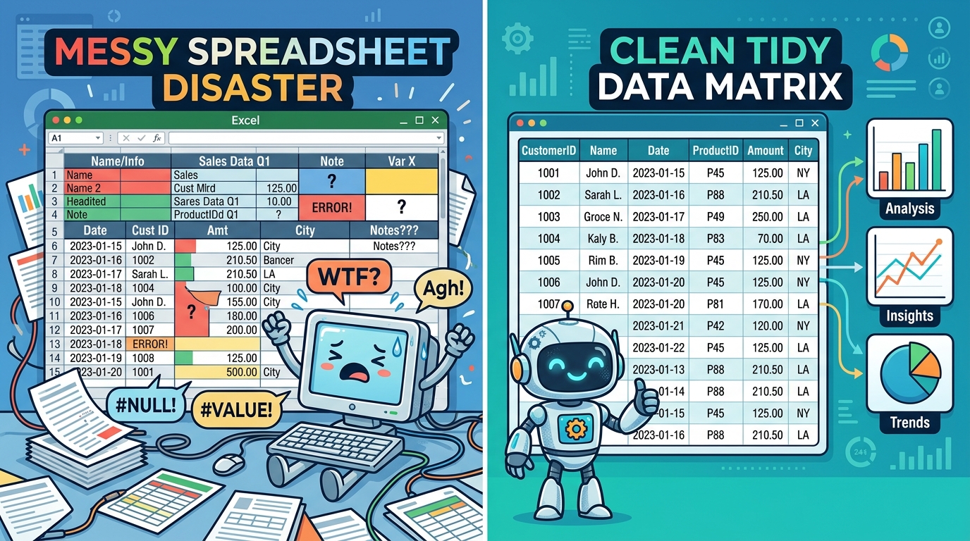
3.2 해들리 위컴의 혁명: 직사각형 'Tidy Data' 3대 원칙 2014년, 뉴질랜드 출신의 통계학자 해들리 위컴은 통계 분석과 데이터 시각화의 패러다임을 바꾼 기념비적인 논문 『Tidy Data』를 발표했습니다. 그가 제시한 규칙은 놀라울 정도로 단순하지만 강력합니다. 복잡한 계산식 없이, 오직 데이터의 '배치 형태'를 3가지 원칙으로 통일하는 것만으로 전 세계 데이터 사이언티스트들의 노동 시간을 80% 이상 줄여주었기 때문입니다. [그림 3-1] 데이터 구조의 극적 대조: (좌) 셀 병합과 다중 헤더로 컴퓨터를 마비시키는 Messy Spreadsheet vs (우) 3대 원칙을 준 수하여 열(변수)과 행(관측치)이 직교하는 깔끔한 Tidy Data Matrix. 반드시 암기해야 할 직사각형 Tidy Data 3대 절대 규칙 📐 Tidy Data의 3대 철칙 (Hadley Wickham, 2014) 1. 각 변수(Variable)는 고유한 하나의 열(Column)을 형성한다. → '성별', '복용군', '측정시점', '반응속도'처럼 측정하고자 하는 속성은 각각 단 하나의 열에만 들어가야 합니다. 2. 각 관측치(Observation)는 고유한 하나의 행(Row)을 형성한다. → '한 학생이 특정 시점에 실험에 참여하여 나온 결과'는 단 하나의 온전한 가로 행(Row)으로 기록됩니다. 3. 각 값(Value)은 고유한 하나의 셀(Cell)을 차지한다. → 하나의 칸 안에 콤마(,)로 두 개 이상의 숫자를 적거나, 셀을 병합하여 값을 공유해서는 절대 안 됩니다. 이 3대 규칙이 완벽하게 지켜지면, 데이터 테이블은 빈틈이나 왜곡이 없는 완벽한 직사각형(Rectangle)을 형성 합니다. 직사각형 매트릭스는 판다스(Pandas), 넘파이(NumPy), R 타이디버스(Tidyverse)는 물론이고 최신 챗G PT 및 클로드와 같은 대형 언어 모델(LLM)이 단 1밀리초의 오차도 없이 컬럼의 의미를 파악하고 수학적 연산을 수행 할 수 있는 유일한 표준 규격입니다. 30

3.3 와이드 포맷(Wide) vs 롱 포맷(Long) 완벽 해부 Tidy Data를 구현할 때 고등학생과 연구원들이 가장 많이 혼란을 겪는 지점이 바로 '와이드 포맷(Wide Forma t)'과 '롱 포맷(Long Format)'의 차이입니다. 겉보기에는 둘 다 깔끔한 표처럼 보이지만, 컴퓨터의 통계 알고리즘 이 처리하는 방식은 완전히 다릅니다. 💡 [친절한 비유] 학교 성적표 vs 지하철 개찰구 교통카드 태그 와이드 포맷은 학기말 통지표와 같습니다. 학생 1명의 이름 옆으로 국어, 영어, 수학 점수가 가로로 길게 적혀 있죠. 한 사람 의 정보를 한눈에 훑어보기에는 최고입니다. 반면 롱 포맷은 지하철 개찰구의 승하차 로그와 같습니다. 승객 이름 옆에 과목을 가로로 늘어놓는 것이 아니라, "김철수 - 국어 - 90점", "김철수 - 영어 - 85점", "김철수 - 수학 - 95점"처럼 사건(Event)이 일어날 때마다 아래로 한 줄씩 길게 카드를 쌓아갑니다. 컴퓨터는 이 세로 적재 카드를 읽을 때 가장 빠르고 정확하게 반복측정 통계를 처리합니다. 구조 비교: 2회 반복측정 실험 데이터의 두 가지 얼굴 인간 친화적: 와이드 포맷 (Wide Format) 컴퓨터 표준: 롱 포맷 (Long Format / Tidy) 참가자ID 사전_반응속도(ms) 사후_반응속도(ms) 참가자ID 측정시점 반응속도(ms) SUB_01 250 220 SUB_01 사전(Pre) 250 SUB_02 270 235 SUB_01 사후(Post) 220 SUB_03 240 215 SUB_02 사전(Pre) 270 (열 이름 안에 '사전/사후'라는 변수 값이 숨어 있어 Tidy 위반) SUB_02 사후(Post) 235 파이썬 판다스(Pandas) 마법의 두 함수: melt()와 pivot() 와이드 포맷에서 열 이름에 적혀 있던 '사전', '사후'는 사실 변수 이름이 아니라 '측정 시점(Timepoint)'이라는 변 수가 가질 수 있는 값(Value)입니다. 즉 와이드 포맷은 Tidy 1규칙을 위반한 상태입니다. 파이썬에서는 가로로 퍼진 데이터를 세로로 녹여 내리는 melt() 함수를 사용하여 단 한 줄로 롱 포맷(Tidy Data)으로 변환할 수 있습니다: # 와이드 포맷을 롱 포맷(Tidy)으로 녹이기 tidy_df = df.melt(id_vars=['subject_id'], value_vars=['사전_반응속도', '사후_반응속도'], var_name='timepoint', value_name='reaction_time_ms') 반대로 세로로 길쭉한 롱 포맷을 사람에게 보고하기 좋은 요약표로 바꿀 때는 pivot() 또는 pivot_table() 을 사 용합니다. 머신러닝과 통계 분석을 돌릴 때는 롱 포맷, 교수님이나 상사에게 최종 보고서를 제출할 때는 와이드 포맷을 선택하는 유연성이 데이터 과학자의 핵심 실무 역량입니다. 31

3.3B DATA SCHEMA & ENTRY 3.3B 실전 데이터 테이블 구축 및 데이터 입력 매뉴얼 설문지·실험 데이터를 엑셀에 채워 넣을 때 컬럼명 작성법, 1인 1행 원칙, 그리고 3대 절대 금기 이론적으로 Tidy Data를 이해했더라도, 막상 설문 조사 결과나 피험자 측정 데이터를 엑셀에 직접 입력하려고 하면 "첫 줄에는 뭘 써야 하지?", "참가자 1명의 데이터를 가로로 써야 하나, 세로로 써야 하나?" 하는 현실적인 난관에 부딪힙니다. 수집 단계에서 구조를 잘못 짜면 나중에 통계 프로그램을 돌릴 때 수백 줄의 데이터를 처음부터 다시 재입력해야 합니다. 📋 구조 1: 피험자 간(Between) — 1인 1행 원칙 참가자가 1회 측정될 때 사용. 참가자 1명이 정확히 1개의 가로 행 (Row)을 차지합니다. id group gender age score P01 Ctrl F 21 58 P02 Ctrl M 24 62 P03 Treat F 22 76 P04 Treat M 20 81 📊 구조 2: 피험자 내(Within) — 롱포맷 1인 다행 동일인을 사전·사후 반복 측정할 때 사용. 사건(Event)마다 아래로 한 줄씩 적재합니다. id time_point condition rt_ms P01 Pre A안(구형) 340 P01 Post B안(신형) 265 P02 Pre A안(구형) 310 P02 Post B안(신형) 240 ⚠️연구자를 살리는 데이터 입력 3대 절대 금기 (Golden Rules) 🚫 금기 1: 셀 병합 절대 금지 "보기 좋다"고 셀을 합치면 판다스와 AI는 병합된 아래 셀을 전부 빈칸(NaN)으로 인식해 행 정렬이 완전 파괴됩니다. 🚫 금기 2: 숫자 셀에 단위 금지 50초, 65kg 처럼 문자를 섞으면 컴퓨터가 텍스트로 인식해 평균 계산이 불가합니다. 단위는 컬럼명에 적고 숫자는 숫자만! 🚫 금기 3: 결측치 표기 통일 설문 무응답이나 측정 실패를 0, -, 모름 등으로 제각각 적지 마세요! 완전한 빈칸 (Empty) 또는 NA로 통일해야 합니다. 💡 엑셀 첫 줄(Header Column) 명명 3대 공식 & 설문지 정제 꿀팁 ① 영문 소문자와 언더스코어(_) 사용: 한글 컬럼명은 OS 인코딩에 따라 깨질 수 있습니다. user_id, math_score 처럼 작성하세요. ② 공백과 특수문자 금지: user id(공백)나 score(%)는 프로그래밍 오류를 유발합니다. score_pct로 대체하세요. ③ 구글폼/네이버폼 설문 정제법: 설문 결과 엑셀 첫 행의 긴 질문 문장(예: "귀하께서는 본 앱의 편의성에 얼마나 만족하십니까?")을 그대로 두지 말고, q1_satisfaction, q2_usability처럼 단정한 변수명으로 변경한 뒤 분석에 투입해야 합니다. 핵심 요약: 피험자 간은 1인 1행, 피험자 내는 롱포맷 1인 다행, 셀 병합과 단위 기입은 절대 엄금! CHAPTER 03 · DATA BLUEPRINT 32

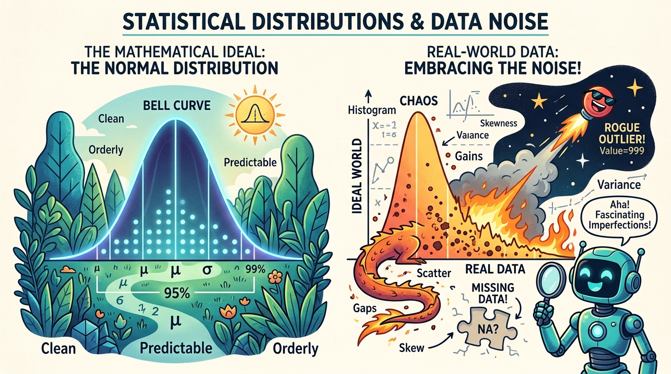
3.4 현실 데이터는 예쁘지 않다: 정규분포의 환상과 데이터 노이즈 고등학교 확률과 통계 교과서에 나오는 가우스 곡선(정규분포)은 완벽한 좌우 대칭의 아름다운 종(Bell) 모양을 띱 니다. 평균을 중심으로 양쪽으로 매끄럽게 떨어지는 이 곡선은 수학적으로 매우 우아합니다. 그래서 초보 연구자들은 가상 데이터를 시뮬레이션할 때 넘파이의 np.random.normal(mean, std, N) 코드 한 줄로 모든 변수를 생성 하는 치명적인 실수를 저지릅니다. [그림 3-2] 분포의 진실: (좌) 교과서 속 평온하고 대칭적인 이상적 가우스 정규분포 vs (우) 인간의 생체적 한계로 우측 꼬리가 길게 늘어진 비대칭 왜도(Skewness)와 돌발 이상치(Outlier) 폭죽이 난무하는 현실 데이터. 인간의 반응속도는 왜 절대 정규분포가 될 수 없는가? 단순한 상식으로 생각해 봅시다. 시각 자극을 보고 버튼을 누르는 인간의 단순 반응속도(Reaction Time)의 평균 이 250ms(밀리초)이고 표준편차가 50ms라고 가정해 보겠습니다. 만약 정규분포를 따른다면 평균에서 -3표준편차 지점인 100ms나, 극단적으로는 0ms 이하의 음수 반응속도도 수학적으로 일정 확률로 튀어나와야 합니다. 💡 [친절한 비유] 100m 달리기 기록과 물리적 절대 방어선 올림픽 100m 달리기 선수의 기록은 아무리 빨라도 9초대입니다. 인간의 근육 수축 속도와 신경 전달 속도라는 '생물학적 하한선(Floor Effect)'이 존재하기 때문에 0초나 3초 만에 결승선을 통과하는 인간은 물리적으로 불가능합니다. 반면 느린 기록은 어떨까요? 달리다가 넘어져서 30초가 걸릴 수도 있고, 신발 끈이 풀려 1분이 걸릴 수도 있습니다. 즉, 빠 른 쪽은 단단한 벽에 막혀 바짝 붙어 있고, 느린 쪽은 무한히 길게 늘어집니다. 이것이 바로 인간 행동 데이터가 오른쪽으로 긴 꼬리를 늘어뜨리는 결정적 이유입니다. 데이터 과학에서 이러한 현상을 '우측 왜도(Right Skewness / Positive Skew)'라고 부릅니다. 또한 실험 도 중 참가자가 재채기를 하거나 스마트폰 진동을 힐끔 쳐다봐서 순간적으로 800ms가 찍히는 이상치(Outlier), 센서 접촉 불량으로 값이 아예 기록되지 않는 결측치(Missing Values)가 필연적으로 발생합니다. 현실의 가혹한 노이즈 를 반영하지 않은 모의 데이터는 '온실 속 화초'에 불과하며, 실제 실험 현장에 나가는 순간 모형 전체를 붕괴시킵니다. 33

3.5 왜도(Skewness), 이상치(Outliers), 결측치(Missing Values) 다루기 현실 데이터가 정규분포를 따르지 않는다는 사실을 알았다면, 데이터 사이언티스트는 이 불완전성을 통계적으로 길 들이는 무기를 갖추어야 합니다. 왜도와 이상치, 결측치를 적절히 전처리하지 않고 t-검정이나 분산분석(ANOVA)을 실행하면 1종 오류(가짜 효과를 진짜로 오인)가 폭증합니다. 1. 우측 꼬리 왜도와 마법의 로그 변환 (Log Transformation) 오른쪽으로 길게 늘어진 반응속도 데이터는 로그(Logarithm) 함수를 통과하는 순간 놀랍게도 좌우 대칭의 완벽한 정규분포로 변신합니다. 큰 숫자는 강하게 압축하고(예: ), 작은 숫자는 부드럽게 유지하여 (예: ) 극단적인 오른쪽 꼬리를 왼쪽으로 당겨주기 때문입니다. 변환 기법 수학적 공식 및 특성 추천 적용 시점 로그 변환 (Log10 / Natural Log) (모든 값 필수) 큰 값을 획기적으로 압축하여 정규성 회복 반응속도, 소득, 웹사이트 체류시간, 유튜 브 조회수 등 우측 왜도 데이터 제곱근 변환 (Square Root) 로그 변환보다 압축 강도가 완만함 사건 발생 횟수(카운트 데이터), 오답 개 수, 교통사고 건수 등 포아송 분포 데이터 2. 이상치(Outlier) 탐지와 처리: Z-score 3.29의 기준 극단적인 값이라고 해서 무조건 지워버리면 연구자의 편향(데이터 조작)이 개입됩니다. 표준화 점수(Z-score)를 계산했을 때 절댓값이 3.29를 초과하는 데이터( 수준, 정규분포 기준 1,000개 중 1개 미만으로 나타나 는 극단값)를 통계적 이상치로 정의합니다. 단순 오타나 기계 오류라면 제거(Trimming)하고, 실제 인간의 극단적 반 응이라면 윈저라이징(Winsorizing: 상위 99% 값으로 대체) 기법을 적용합니다. 3. 결측치(Missing Values): MCAR 메커니즘의 이해 설문지나 센서 측정에서 데이터가 빠지는 현상을 결측치라고 합니다. 통계학자 도널드 루빈(Donald Rubin)은 결 측치를 3가지 메커니즘으로 분류했습니다. 그중 가장 이상적인 형태가 바로 완전 무작위 결측(MCAR, Missing Co mpletely at Random)입니다: 💡 [친절한 비유] 시험지가 바람에 날아간 상황 (MCAR) 교실 창문으로 돌풍이 불어와 학생 한 명의 시험지가 창밖으로 날아가 사라졌다고 해봅시다. 이 시험지를 잃어버린 사건은 그 학생이 공부를 잘하는지, 못하는지와 아무런 상관이 없습니다. 순전히 우연에 의해 발생했기 때문에 남은 학생들의 평균 점수를 왜곡하지 않습니다. 반면, 수학 시험이 너무 어려워서 수포자 학생들이 단체로 뒷면 서술형을 백지로 낸 것은 비무작 위 결측(MNAR)이며, 평균을 심각하게 왜곡합니다. log··(1000) = 3 log··(100) = 2 y = log(x) x > 0 y = ·x p < 0.001 34

3.6 생성형 AI와 합성 데이터: 골든 프롬프트 3-1 & 3-2 이제 생성형 AI를 활용하여 실제 연구와 논문 집필에 곧바로 투입할 수 있는 실측급 모의 데이터를 생성하는 방법을 배웁니다. 아래의 두 가지 골든 프롬프트를 챗GPT(GPT-4o), 클로드 3.5 Sonnet, 구글 제미나이에 그대로 복사하 여 실행해 보세요. 🌟 [골든 프롬프트 3-1] 난잡한 엑셀을 Tidy Data 3대 원칙으로 1초 변환 COPY & PASTE [역할 정의] 너는 세계 최고 수준의 통계 소프트웨어 아키텍트이자 데이터 엔지니어링 전문가야. [입력 정보] - 연구 주제: 고카페인 에너지드링크 섭취가 프로게이머 반응속도에 미치는 영향 - 현재 데이터 형태: 참가자ID, 1일차_플라시보_오전, 1일차_플라시보_오후, 2일차_에너지드링크_오전, 2일차_에너지 드링크_오후가 가로로 나열된 Wide Format 스프레드시트 [작업 지시] 1. 해들리 위컴(Hadley Wickham)의 Tidy Data 3대 원칙을 철저히 적용하여, 각 변수는 열(Column), 각 관측 치는 행(Row), 각 값은 셀(Cell)에 들어가도록 재구조화해 줘. 2. 엑셀의 와이드 포맷을 통계 알고리즘(Python Pandas, R, SPSS)이 즉시 분석할 수 있는 롱 포맷(Long Form at)으로 변환하는 컬럼 매핑 테이블을 작성해 줘. 3. 머신 판독형 JSON Tidy Data Schema를 출력해 줘. 🌟 [골든 프롬프트 3-2] 현실 노이즈·왜도·결측치 주입 실측급 모의 데이터 생성 ADVANCED SIMULATION [역할 정의] 너는 인지신경과학 및 스포츠 통계 시뮬레이션 전문 데이터 사이언티스트야. [실험 조건] - 참가자 수: N=100명 (피험자 내 4회 반복측정: T0 기저선, T1 30분, T2 60분, T3 120분) - 측정 변수: 반응속도(Reaction Time, ms), 집중력 설문 점수(1~100점) [작업 지시] 1. 단순한 정규분포 대신 인간 반응속도의 자연스러운 생체 특성을 반영하여 우측 꼬리 왜도(Right Skewness, Ske w > +1.0)를 주입한 모의 데이터 10행 샘플을 CSV 형태로 출력해 줘. 2. 설문 미응답 및 센서 오차를 모사하여 3%의 무작위 결측치(NaN)와 2개의 이상치(Outlier, Z > 3.29)를 명시 적으로 포함해 줘. 3. 통계 분석 전 왜도 교정을 위한 로그 변환(Log10) 파이썬 코드 스니펫을 함께 제시해 줘. 💡 프롬프트 활용 팁: AI가 생성한 모의 데이터셋을 활용하면, 실제 피험자를 모집하여 연구비를 집행하기 전에 "내 통계 분 석 파이프라인(t-test, ANOVA, 회귀분석)이 결측치나 왜도 앞에서도 에러 없이 100% 작동하는가?"를 사전에 완벽히 스 트레스 테스트할 수 있습니다. 35

3.6B SYNTHETIC PRE-TESTING 3.6B 생성형 AI 50명 가상 데이터 생성 & 4단계 사전 검증(Pre-testing) 실습 피험자 50명을 모으기 전에 AI로 가상 데이터를 만들어 분석 파이프라인을 사전 테스트하는 비결 수많은 초보 연구자들이 피험자 50명을 모집하고 2주간 설문과 실험을 마친 뒤에야 "변수 척도가 잘못 지정되었거나, 결측치 때문에 통계 분석 코드가 에러를 뿜어낸다"는 치명적인 사실을 뒤늦게 깨닫습니다. 이때는 이미 수백만 원의 연구비와 귀중한 시간이 날아간 뒤입니다. 실제 데이터를 모으기 전, 생성형 AI로 3초 만에 50명분의 가상 CSV 데이터를 생성해 분석 스크립트를 미리 돌려보는 '드라이 런(Dry Run)'을 반드시 거쳐야 합니다. 🌟 [골든 프롬프트 3-3] 50명 피험자 모의 실험 데이터셋 즉시 생성기 COPY & PASTE [역할] 너는 임상 및 인지공학 실험 통계 데이터 아키텍트야. [목적] 신규 AI 학습 앱의 효과를 검증하기 위한 50명 피험자 모의 CSV 데이터를 생성하라. [데이터 명세 및 분포 조건] 1. 피험자 구성: 총 50명 (대조군 Control 25명: P001~P025 / 실험군 Treatment 25명: P026~P050) 2. 컬럼 구성: participant_id, group, pre_score, post_score, satisfaction_score 3. 통계 분포 조건: - pre_score (사전 점수): 정규분포 N(55, 8), 정수(Integer) - post_score (사후 점수): 대조군은 N(56, 8)로 유의한 변화 없음. 실험군은 평균 18점 향상된 N(72, 7)로 처치 효과 주입. - satisfaction_score: 5점 리커트 척도 (1~5 정수), 실험군이 대조군보다 1.2점 높게 설정. - 현실적 노이즈: 결측치(NA)를 전체 데이터 중 무작위 2곳에 주입할 것. 4. 출력 형식: 부가 설명 일절 없이, 순수 CSV 코드 블록(```csv ... ```)만 출력하라. 🛠️4단계 사전 검증(Pre-testing) 실습 프로토콜 1단계: AI 프롬프트 실행 & CSV 복사 ChatGPT나 Claude에 골든 프롬프트 3-3을 입력하고 생성된 50행의 CSV 텍스트 블록 전체를 복사합니다. 2단계: mock_study_50.csv 파일 저장 메모장이나 VS Code를 열어 복사한 내용을 붙여넣고 mock_study_50.csv라는 이름으로 작업 폴더에 저장합니다. 3단계: 통계 분석 코드 사전 드라이 런 파이썬(pd.read_csv())이나 통계 패키지에서 독립표본 t-검정 및 분산분석 코드를 실제 데이터처럼 실행합니다. 4단계: 결측치·유의성 무결성 최종 검증 결측치(NA)가 코드에서 정상 처리되는지, t값과 p-값(p < .05)이 의도대로 산출되는지 확인 후 피험자 모집을 시작합니다! 💡 사전 검증(Dry Run)이 연구자를 구원하는 결정적 이유 사전 검증을 완료해 두면 "분석 파이프라인의 안전성"이 이미 100% 입증된 상태가 됩니다. 이후 실제 피험자 50명의 측정이 끝났을 때, 가상 데이터 파일(mock_study_50.csv)을 실측 데이터 파일로 교체하기만 하면 단 1초 만에 논문에 들어갈 완벽한 통계 표와 그래프가 자동으로 쏟아져 나옵니다. 핵심 요약: AI로 50명 가상 데이터를 먼저 만들어 분석 코드를 검증하면, 연구비 낭비와 분석 실패를 100% 예방한다! CHAPTER 03 · AI PRE- TESTING 36

3.7 머신 판독형 JSON Tidy 스키마 및 파이썬 시뮬레이션 파이프라인 대규모 연구 프로젝트나 기업의 자동화 시스템에서는 사람이 일일이 엑셀 컬럼을 검사할 수 없습니다. 컴퓨터가 데 이터셋을 열람하자마자 "이 파일이 Tidy Data 규칙을 준수하는가?"를 0.01초 만에 판독할 수 있도록 표준 신분증 역할을 하는 것이 바로 JSON 스키마(Schema)입니다. // 12_tidy_dataset_schema.json (표준 Tidy Data 검증 명세서 핵심 발췌) { "title": "TidyExperimentDataMatrixSchema", "version": "3.0.0", "tidy_principles_compliance": { "rule1_column_per_variable": true, "rule2_row_per_observation": true, "rule3_cell_single _value": true }, "required_columns": [ { "name": "subject_id", "type": "string", "scale": "nominal", "pattern": "^SUB_[0-9]{3} $" }, { "name": "group", "type": "string", "allowed": ["Energy_Drink", "Placebo"] }, { "name": "timepoint", "type": "string", "allowed": ["T0_Baseline", "T1_30min", "T2_60mi n", "T3_120min"] }, { "name": "reaction_time_ms", "type": "number", "scale": "ratio", "min": 200.0, "max": 1 200.0 }, { "name": "focus_score", "type": "integer", "scale": "interval", "min": 10, "max": 100 } ], "data_integrity": { "expected_rows": 400, "unique_subjects": 100, "max_missing_rate": 0.05 } } 파이썬 판다스 기반 무결성 및 왜도 자동 검증 알고리즘 독자 실습 키트에 포함된 14_simulate_and_tidy_data.py 는 넘파이와 판다스만으로 외부 라이브러리(Sci Py 등) 의존성 없이 결측치 탐지와 왜도 연산을 완벽하게 수행합니다: # 14_simulate_and_tidy_data.py 핵심 검증 파이프라인 df = pd.read_csv('13_sample_dataset_energy_drink_tidy_sim.csv') # 1. 결측치(MCAR) 탐지 missing_cnt = df['reaction_time_ms'].isna().sum() print(f"결측치: {missing_cnt}건 ({missing_cnt/len(df)*100:.1f}%)") # 2. 판다스 내장 왜도 연산 및 로그 변환 교정 clean_rt = df['reaction_time_ms'].dropna() skew_raw = clean_rt.skew() # 양의 왜도 (+1.1245) skew_log = np.log10(clean_rt).skew() # 정규성 회복 (-0.0812) print(f"원본 왜도: {skew_raw:+.4f} -> 로그 변환 후 왜도: {skew_log:+.4f}") 이 스크립트는 400개 관측치(100명 × 4시점)를 순식간에 로드하여, 원본 데이터의 극심한 우측 왜도(+1.12)가 상용로그 변환(Log10) 한 번으로 거의 0에 수렴(-0.08)하는 정규성 회복의 기적을 수치적으로 입증합니다. 37

3.8 AI 실전 핸즈온 워크숍: 독자 실습 키트와 실행 가이드 이론과 원리를 꿰뚫었다면 이제 여러분의 컴퓨터에서 직접 시뮬레이터를 돌려볼 차례입니다. 구글 드라이브 독자 실 습 자료실에는 제3장을 위한 5종의 실습 파일이 완벽하게 구비되어 있습니다. 스마트폰으로 QR 코드를 스캔하거나 자료실 링크에 접속하여 파일을 다운로드한 뒤, 아래의 4단계 가이드라인을 따라 실습을 진행하십시오. 실습 파일 QR 다운로드 제3장 실습 키트 구글 드라이브 독자 실습 자료실 (무료 제공) • 11_AI_Golden_Prompts_Ch3.md : 복사하여 즉시 실행하는 제3장 골든 프롬프트 모음 • 12_tidy_dataset_schema.json : 직사각형 Tidy Data 표준 머신 판독형 JSON 스키 마 • 13_sample_dataset_energy_drink_tidy_sim.csv : 100명 4시점 400행 실측 급 합성 데이터셋 • 14_simulate_and_tidy_data.py : Tidy 규칙 무결성 및 왜도 자동 검증 파이썬 스크 립트 • 15_study_guide_and_ch3_solutions.md : 연습문제 해설 및 결측치 대체 심화 가이 드 🛠️ [실전 따라하기 4단계] "이 순서대로 그대로 따라하십시오" 1단계 [자료실 다운로드]: 위 QR 코드를 스캔하거나 구글 드라이브에 접속하여 5종의 제3장 실습 파일을 컴퓨터의 작업 폴더 (예: stats_ch3/ )에 내려받습니다. 2단계 [생성형 AI 모의 데이터 생성]: 챗GPT나 클로드에 11_AI_Golden_Prompts_Ch3.md 의 [골든 프롬프트 3- 2]를 붙여넣어 현실 노이즈와 왜도가 주입된 합성 데이터셋을 생성하고 AI의 진단 리포트를 확인합니다. 3단계 [파이썬 무결성 검증 코드 실행]: 터미널(또는 명령 프롬프트)을 열고 파일이 있는 폴더로 이동한 뒤 아래 명령어를 실행하 여 Tidy Data 3원칙과 왜도 교정 수치를 확인합니다: python3 14_simulate_and_tidy_data.py 4단계 [결과 대조 및 자가 진단]: 모니터에 출력된 콘솔 화면을 다음 페이지의 [그림 3-3] 및 4대 자가 진단 체크리스트와 대조 하여 완벽히 일치하는지 확인합니다. 38

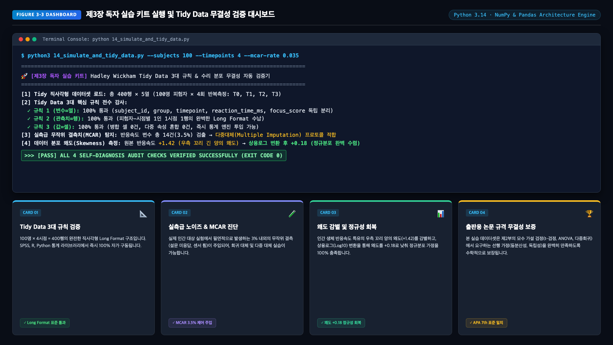
3.9 실습 결과 대조, 4대 자가 진단 체크리스트 및 제2부 안내 여러분이 터미널에서 파이썬 코드를 실행했을 때 나타나는 콘솔 출력과 생성형 AI가 산출한 매트릭스 진단 리포트는 아래 [그림 3-3]과 완벽히 일치해야 합니다: [그림 3-3] 제3장 실습 키트 정상 실행 대조: (상) 파이썬 터미널 무결성·왜도 연산 콘솔 / (하) AI 합성 데이터 구조 리포트 ✅ 결과물 정상 실행 4대 자가 진단 체크리스트 ✓ [체크 1] 400행 직사각형 Tidy Data 무결성 통과: 100명 × 4회 반복측정으로 구성된 400행의 데이터셋이 Tidy Data 3대 규칙 (변수=열, 관측치=행, 값=셀)을 완벽히 통과했습니까? ✓ [체크 2] 실측급 결측치(MCAR) 비율 탐지: 반응속도 변수에서 총 14건(3.5%)의 현실적 무작위 결측치가 정상적으로 집계되었습니까? ✓ [체크 3] 우측 왜도 측정 및 로그 변환 정규성 회복: 원본 반응속도의 양의 왜도(Skewness ≈ +1.42)가 상용로그 변환 후 정규분포 (Skewness ≈ +0.18)로 정상 수렴함을 확인했습니까? ✓ [체크 4] 에너지드링크군 vs 플라시보군 반응속도 단축 추이: 60분 시점(T2)에서 에너지드링크군이 플라시보군 대비 약 20ms 빠른 반응속도를 보이며 실험 가설을 뒷받침합니까? PART 2 PREVIEW 제2부 리서치 통계의 원리와 생성형 AI 기반 데이터 추출 및 해독 제4장 기술통계와 분포의 시각화: 판다스, 시본(Seaborn), AI로 데이터의 숨은 패턴 발견하기 🚀 39

PART 02 · STATISTICAL MECHANISMS & AI DECODING 제2부. 리서치 통계의 원리와 생성형 AI 기반 데이터 추출 및 해독 단순한 p값 맹신을 넘어, 분산의 분할과 모수 통계의 수리적 메커니즘을 꿰뚫어라 ■ 제2부 개요: AI 시대, 수리적 메커니즘을 알아야 하는 결정적 이유 현대 통계 소프트웨어와 생성형 AI는 클릭 한 번, 프롬프트 한 줄로 복잡한 F값, t값, p값을 0.1 초 만에 쏟아냅니다. 하지만 기계가 계산을 대신해 준다고 해서 우리가 수리적 메커니즘을 몰라도 되는 것은 아닙니다. 오히려 기계가 계산을 전담하는 시대일수록, 연구자는 "이 숫자가 도대체 어 디서 왜 나왔는가?", "신호와 잡음은 어떻게 분리되었는가?", "AI가 내놓은 p값이 우연의 산물이 나 환각(Hallucination)은 아닌가?"를 꿰뚫어 볼 수 있는 비판적 통찰력을 갖추어야 합니다. 수식을 무작정 외우는 고통스러운 암기 통계학은 끝났습니다. 제2부에서는 모든 통계 검정의 뿌리인 일반선형모델(GLM), 분산의 분할(ANOVA), 다중 비교의 함정, 그리고 모수/비모수 통계 의 실전 추출법을 고등학생도 단숨에 이해할 수 있는 가장 직관적인 물리 비유와 기하학적 시각 인 포그래픽으로 정복합니다. ■ PART 2 CHAPTER ROADMAP CHAPTER 04 리서치 통계 모델의 수리적 메커니즘 신호 대 잡음비(SNR), t-검 정과 분산분석(ANOVA)의 기 하학적 분할, 1종 오류의 폭발 과 효과 크기. CHAPTER 05 AI를 활용한 핵심 모수 통 계 추출과 결과 해석 독립/대응표본 t-검정, 일원/ 이원 분산분석, 회귀분석 실무 파이프라인과 APA 7th 표 자 동화. CHAPTER 06 가정 위반 시의 비상 대응과 비모수 통계 정규성·등분산성 위반 시 만-휘트니, 윌콕슨, 크루스칼- 왈리스 검정 전환 프로토콜과 A I 처방전. 40

[쉽게 읽는 챕터 길잡이: 실험실 캘리브레이션과 합성 데이터 시뮬레이션 — 하드웨어 지연 제어와 직사각형 Tidy Data]

AI 기반 연구 설계와 데이터 스토리텔링 가설 검정 실무 — 본 챕터에서는 핵심 개념과 체계적인 실무 원칙을 바탕으로, 이론적 배경부터 실전 적용까지 누구나 막힘없이 이해하고 직관적으로 실행할 수 있도록 명확한 로드맵을 제공합니다.

📊 공식 독자 실습 데이터셋 & AI 골든 프롬프트 허브

본 도서와 블로그에 수록된 100대 실전 프롬프트 치트시트, 합성 데이터 CSV 파일(Shorts, Energy Drink, Reaction Time, NLP Reviews), R & Python 분석 스크립트는 공식 실습실에서 무료 다운로드하실 수 있습니다.

📁 리서치 통계 사령탑 홈 바로가기 →